Output document in YAML

You can change the output: html_document, to output: github_document, to output: word_document, to output: pdf_document. If you are having trouble with the pdf_document output, this means that the LaTeX¹ engine is not installed on your computer. For this I am borrowing instructions from here where they suggest these links:

• For Windows: Go to https://miktex.org/howto/install-miktex and follow directions to install MikTex.
• For Mac: Go to https://tug.org/mactex/mactex-download.html and follow directions to install MacTex.

In the YAML, one puts some broad instructions on how Pandoc needs to interpret the document, one big information being the output. You can see right away that with just one document, you can create at least 4 different documents. when you typed output: github_document, there was an html preview that popped-up, but in the background, a *.md file was created. This *.md* file is interpreted by GitHub to render the document within the GitHub environment. If you try to click on a *.html file that is hosted on GitHub, only code will appear, and not the rendered html document.

Table Of Content

R markdown provides the possibility of Table Of Content or toc that you put as a variable in the YAML part of the R Markdown. The toc will appear at the head of the document and will give you links to all the heading levels you have created. This is very useful to quickly give you an outline of your document and allows you to get directly to the section of your choice. The YAML of this document is

---
title: "Crash course on R Markdown"
author: "François Birgand"
date: "09/10/2017"
output: 
  html_document:
    toc: true
    toc_float: true
bibliography: RMD_course_bibtex.bibtex
link-citations: true
csl: journal-of-hydrology.csl
---

Notice that the html_document has now been put on another line for organization purposes, but also note that a : has been added at the end of html_document:. This tells Pandoc that among the html_document, a toc should be added.

Bibliography

I have created and maintained for over 15 years a database written in Microsoft Access of around 2000 articles, most of them photocopied and typed in the database by hand during and after my Ph.D. (yes, I should have a medal!…) but I have to admit that this system is past its time… I have now switched to Paperpile. There are many other referencing software out there now (a list and comparison can be found here). The beauty of them is that they will all export in recognized formats and this is what we care about here. So no more copy/paste of references from some pdf. We are going into reproducible research. This means that all the articles you want to work with will be entered in the reference database of your choice. Make sure you start one ASAP!

In the YAML header, you can now see bibliography: RMD_course_bibtex.bibtex. This means that there is a file named RMD_course_bibtex.bibtex that is located in the same directory as the .Rmd file, which when we ‘knit’, Pandoc will look for. You can access this .bibtex file in the GitHub directory. There is actually a possibility to add within the .Rmd document itself, the text needed for Pandoc to read the references, but unless you only have very few references, this can become very messy quickly. See the RStudio Bibliographies documentation for more details.

In short, in this file, there is a list of articles which information is coded according to the format chosen. By the way, a lot of the details for the bibliography are available on the RStudio Bibliographies documentation. R Markdown will recognize up to 10 different formats. The one Paperpile exports is .bibtex, so this is the one I have have added in the YAML header. The filename extension will determine the rendering process, so make sure you have the right extension as well.

So, in the .bibtex file I have, the first article appears as

@ARTICLE{Kuhne2009-tn,
  title   = "Improving the Traditional Information Management in Natural
  Sciences",
  author  = "K{\"u}hne, Martin and Liehr, Andreas W",
  journal = "Data Sci. J.",
  volume  =  8,
  pages   = "18--26",
  year    =  2009,
  issn    = "1683-1470, 0308-9541",
  doi     = "10.2481/dsj.8.18"
}

The first item after “ARTICLE{” is the unique identifier for the article. The identifier of this article is Kuhne2009-tn. When one wants to cite this article, one will say something like “reproducible research has been suggested to become the norm²”. And you would code like

"reproducible research has been suggested to become the norm [@Kuhne2009-tn]"

If you want to say that “Kühne et al.² have shown that etc.”, you would add a “dash” just before the “@” and code it as such:

Kühne et al. [-@Kuhne2009-tn] have shown that etc."

If you want to cite several references, you would add a semicolon between the two such as in:

"reproducible research has been suggested to become the norm [@Kuhne2009-tn; @Buckheit1995-ls]"

Notice that among all the fields from the example above, there are doi and issn. doi stands for “Digital Object Identifier”. issn stands for International Standard Serial Number (ISSN), which is an eight-digit serial number used to uniquely identify a serial publication. The doi value in this example is 10.2481/dsj.8.18, which is unique in the world. These doi are applied to articles but not only. They are also applied to data. Eventually, all data that will be used in an article will have to have its own doi and all the codes that are used to analyze the data will refer to this unique doi. This is not quite implemented yet (in 2017), but will likely be by 2022. doi or url (not added here; stands for Uniform Resource Locator. Quite a mouthful, really, for what it is: a web address) are not necessarily exported from your reference software by default. Make sure you add this possibility, as doi is almost routinely added in the reference list in most journals.

The reference list of the citations will appear right after you place

# References

at the bottom of your Rmd docucment. When rendering your document, the list will appear automatically afterwards, and if you have in text notes, these will appear underneath.

Link to citations

One very nice feature is to create hyperlinks from the in-text citations to the citations in the reference section. For this, just add link-citations: true in the YAML header.

CSL and styling of citations

CSL stands for Citation Style Language. The CSL line command is an option for the citation styles to be used in your document. You can comment it out by adding a “#” in front of it and the default .CSL file will apply without you noticing it. Each journal has its own way of handling how an article/reference should be cited in the text, and in the reference section, and there are hundreds of different styles out there… You can read lots of details on this CSL primer about how all this works.

While I was writing this tutorial, I did not specify at first the citation style. And I kept getting, using the same example as before, “(Kühne and Liehr 2009)”, although I wanted “(Kühne and Liehr, 2009)”, i.e., with a comma between the authors and the date, because this is the way I always did it and I think it is a lot better this way. Then I started thinking about the journals for which the inline citations are numbers, sometimes in brackets, sometimes without brackets… what a nightmare…! Actually it is extremely simple: all this is done automatically when you specify the CSL corresponding to the journal style following which you wish to write.

For this, you can pick at https://github.com/citation-style-language/styles the *.CSL file you are looking for (actually there are too many of them and they are not all displayed). The fastest way is to Google “ CSL”, and you will land on the CSL file you are looking for. I recommend that you click on the raw icon on GitHub, and copy all the file in a text editor. Warning! You need to make sure that your text editor does not add any weird formatting or add an extension at the end of the file. I had that problem and I could not see the extension on my computer, although I had the option to display so. Save the file in the same directory as your .Rmd.

So, to go back with my struggling to style the inline citation and the “missing comma”, it turns out that the default CSL file uses a “Chicago author-date format” (I am not sure what this means exactly), which in text styling is “(author date)”, without the comma…! If you use “journal-of-hydrology.CSL”, you will see that all of a sudden after you knit, the commas just appeared…! Eureka! If you use “nature.CSL” (because we all want to be ready when we publish in Nature!), you will see that there are no more in-line citations, just numbers in superscript, hyphenated when needed, and the references are all in order, with the journal names in italics, the journal volume in bold, the year in parenthesis at the end, etc.! Is not that wonderful? Without your doing anything, other than adding the citation properly in the text following the guidelines above.

You can, if you want and have a lot of time to waste, take existing CSL files and modify them to have your own custom citation style. Make sure you take an “independent” CSL file and modify it. Most of them are dependent upon a “source” or independent one, and the code in the CSL file is just saying how the dependent file should slightly alter the independent one. Good instructions on how to do this can be found on the excellent CSL primer.

Paragraph Breaks and Forced Line Breaks

To insert a break between paragraphs, include a single completely blank line.

To force a line break, put two blank spaces at the end of a line.

To insert a break between paragraphs, include a single completely blank line.

To force a line break, put _two_ blank spaces at the end of a line.

Headers

The character # at the beginning of a line means that the rest of the line is interpreted as a section header. The number of #s at the beginning of the line indicates the level of the section (1,2,3, etc.). For instance, Components of R Markdown above is preceded by a single #, because it is of level 1 but Headers at the start of this paragraph is preceded by ### because it is of level 3. Up to six levels are understood by Markdown. Do not interrupt these headers by line-breaks. Make sure that in your .Rmd file, you leave a blank line before a header, otherwise, pandoc will not render it as a header.

Italics and bold

*italics* and _italics_

renders italics and italics

**bold** and __bold__

renders bold and bold

Supbscripts and superscripts

To write sub- and superscripts, like in NO₃^- or PO₄^3- write as

NO~3~^-^ or PO~4~^3-^

PO₄^3- does not look as neat as \(PO_4^{3-}\)

PO~4~^3-^ does not look as neat as $PO_4^{3-}$

but looks more seamless in a normal text because the former does not appear as an equation while the other does.

Lists

* unordered list
* item 2
    + sub-item 1                #4 <spaces> before +
    + sub-item 2                #4 <spaces> before +

• unordered list
• item 2
  • sub-item 1
  • sub-item 2

1. ordered list
2. item 2
    + sub-item 1                #4 <spaces> before +
    + sub-item 2                #4 <spaces> before +

1. ordered list
2. item 2
   • sub-item 1
   • sub-item 2

In the ordered list, there is a subtlety unrevealed in the Rmardown documentation, which is that the numbering always increases, and that only the number value of the first item matters. So, one cannot have a list in a decreasing order (which is too bad because when one makes a list of his/her publications, it is nice to have a decreasing order…), and the only number that matters is the first one. So this code

5. ordered list
7. item 2
2. item 2
                                # blank line for list to take into effect
    b. sub-item 1               #4 <spaces> before b
    a. sub-item 2  

renders this:

5. ordered list
6. item 2

7. item 2

   2. sub-item 1
      
   3. sub-item 2

Quotations

R Markdown is, in particular, both “free as in beer” (you will never pay a dollar for software to use it) and “free as in speech” (the specification is completely open to all to inspect).

Is a quotation from Dr Shalizi which code starts with a >

> R Markdown is, in particular, both "free as in beer" etc.

Computer type

This is to differentiate regular text from code text so that both can be easily differentiated: R vs R.

This is to differentiate regular text from `code text` so that both can be easily differentiated: `R` vs R.

An entire paragraph of code which is rendered as a “code box” in html (but not in pdf) starts with three “back-ticks”, and end the same

Symbols and Special characters

The principal keys, like the alphabet, are understood univocally across platforms such as Windows, Mac OS, or Linux. However, there are special characters such °, ² or µ that have different embedded codes across the different platforms. For example, if you and your co-worker work on the same document and one works using Windows and the other uses Mac, the actual symbol in the code text may not show the same one from one to the other plateform.

For example, if I write in an R markdown document “10 m²” and I have added the ² symbol by typing on a PC “Alt+0178”, as this corresponds to the ascii code for ² in Windows, the same document open on a Mac will render “10 m?”, because it cannot interpret the embedded code for ²…

Several consequences:

1. NEVER use special characters in variable names in an R code,
2. in an R markdown document, use the HTML Number or HTML name in the text

HTML Number and Names can be found on this ascii page

So to type T°C, m² or µm you type like this

So to type T°C, m² or µm you type like this

Do not forget to add the “;” !!!

Absolute Links

a link within the text as a [link](www.rstudio.com)

a link within the text as a link. Absolute links to images, see Images below.

Links within the document

If you want to provide a link back to an existing heading like [The 'R twist' of Mardown: R Markdown](#the-r-twist-of-markdown-r-markdown), you type it as below

So in the [link example](#link_ref) example above point to the absolute link example, the code is like that.

<a id="link_ref"></a>

Footnotes

You can add footnotes in the text by adding [^footnote] right next to the word concerned and add the [^footnote]: with the text next to it JUST BEFORE the # References section.

Images

To add images in a document, add a ! in front of the same syntax as for links such as:

![](https://www.bae.ncsu.edu/wp-content/themes/riddick/dist/images/ncstate-logos/ncstate-brick-2x2-red.png)

to render:

You can modify the width of the image by adding e.g., {width = 50%} to have the image take 50% of the width of the page

![](https://www.bae.ncsu.edu/wp-content/themes/riddick/dist/images/ncstate-logos/ncstate-brick-2x2-red.png){width=50%}

to render:

To align the image, there is no native way of doing it in Markdown, so you can use a little bit of HTML code like <center> ... </center> such as below. Apparently, it might not work that great in html5 though…

<center>![](https://www.bae.ncsu.edu/wp-content/themes/riddick/dist/images/ncstate-logos/ncstate-brick-2x2-red.png){width=25%}</center>

to render:

You can add a caption by just adding the “Using a caption this time” in the brackets.

Using a caption this time

![Using a caption this time ](https://www.bae.ncsu.edu/wp-content/themes/riddick/dist/images/ncstate-logos/ncstate-brick-2x2-red.png){width=33%}

Now, you can add an image in the text like this and it will work just fine.

Now, you can add an image in the text like this ![Using a caption this time](https://www.bae.ncsu.edu/wp-content/themes/riddick/dist/images/ncstate-logos/ncstate-brick-2x2-red.png){width=33%} and it will work just fine. 

However, you can see that the caption was not added. So for the caption to be added, there needs to be a return before and after the image code. If you include the image like this

The caption does not appear.

However, you can see that the caption was not added. So for the caption to be added, there needs to be a return before and after the image code. If you include the image like this
![Using a caption this time](https://www.bae.ncsu.edu/wp-content/themes/riddick/dist/images/ncstate-logos/ncstate-brick-2x2-red.png){width=33%}  
The caption does not appear.

But if you leave a blank line before and after like this

Using a caption this time

The caption will appear.

But if you leave a blank line before and after like this 

![Using a caption this time](https://www.bae.ncsu.edu/wp-content/themes/riddick/dist/images/ncstate-logos/ncstate-brick-2x2-red.png){width=33%}

The caption will appear.

Now if you want to center both figure and caption, you need to add <center> a blank line, the image code, a blank line, then </center>, and it will appear like this:

Using a caption this time

<center>

![*__Using a caption this time__*](https://www.bae.ncsu.edu/wp-content/themes/riddick/dist/images/ncstate-logos/ncstate-brick-2x2-red.png){width=33%}

</center>

And you can see that adding *__ __* aound the caption text put the caption in bold and italic as well.

To have an image linked to a particular website, you can use this code:

[![caption](https://www.bae.ncsu.edu/wp-content/themes/riddick/dist/images/ncstate-logos/ncstate-brick-2x2-red.png)](https://www.bae.ncsu.edu/wp-content/themes/riddick/dist/images/ncstate-logos/ncstate-brick-2x2-red.png)

If you do that, however, the caption will not show any more, even though you have the proper number of lines before and after. If you want a caption below with a link, you will have to add this underneath. So if you want both the image and the caption to have clickable links, and centered like this

you would write:

<center>

[![](https://www.bae.ncsu.edu/wp-content/themes/riddick/dist/images/ncstate-logos/ncstate-brick-2x2-red.png){width=33%}](https://www.bae.ncsu.edu/wp-content/themes/riddick/dist/images/ncstate-logos/ncstate-brick-2x2-red.png)

[This is the corresponding clickable caption I want](https://www.bae.ncsu.edu/wp-content/themes/riddick/dist/images/ncstate-logos/ncstate-brick-2x2-red.png)

</center>

Inline equations

Inline math is marked off witha pair of dollar signs ($), as \(\pi r^2\) or \(e^{i\pi}\).

Inline math is marked off witha pair of dollar
signs (`$`), as $\pi r^2$ or $e^{i\pi}$.

Set off equations

Mathematical displays are marked off with \[ and \], as in \[ e^{i \pi} = -1 \]

Mathematical displays are marked off with `\[` and `\]`, as in
\[
e^{i \pi} = -1
\]

Once your text has entered math mode, R Markdown turns over the job of converting your text into math to a different program, called LaTeX. This is the most common system for typesetting mathematical documents throughout the sciences, and has been for decades. It is extremely powerful, stable, available on basically every computer, and completely free. It is also, in its full power, pretty complicated. Fortunately, the most useful bits, for our purposes, are actually rather straightforward.

Elements of Math Mode

• Most letters will be rendered in italics (compare: a vs. a vs. \(a\); only the last is in math mode, i.e., $a$). The spacing between letters also follows the conventions for math, so don’t treat it as just another way of getting italics. (Compare speed, in simple italics, with \(speed\), in math mode, i.e., $speed$)
• Greek letters can be accessed with the slash in front of their names, as \alpha for \(\alpha\). Making the first letter upper case gives the upper-case letter, as in \Gamma for \(\Gamma\) vs. \gamma for \(\gamma\). (Upper-case alpha and beta are the same as Roman A and B, so no special commands for them.)
• There are other “slashed” (or “escaped”) commands for other mathematical symbols:
  • \times for \(\times\)
  • \cdot for \(\cdot\)
  • \leq and \geq for \(\leq\) and \(\geq\)
  • \subset and \subseteq for \(\subset\) and \(\subseteq\)
  • \leftarrow, \rightarrow, \Leftarrow, \Rightarrow, \rightleftharpoons for \(\leftarrow\), \(\rightarrow\), \(\Leftarrow\), \(\Rightarrow\), \(\rightleftharpoons\)
  • \approx, \sim, \equiv for \(\approx\), \(\sim\), \(\equiv\)
  • See, e.g., http://web.ift.uib.no/Teori/KURS/WRK/TeX/symALL.html for a fuller listing of available symbols. (http://tug.ctan.org/info/symbols/comprehensive/symbols-a4.pdf lists all symbols available in LaTeX, including many non-mathematical special chracters)
• Subscripts go after an underscore character, _, and superscripts go after a caret, ^, as \beta_1 for \(\beta_1\) or a^2 for \(a^2\).
• Curly braces are used to create groupings that should be kept together, e.g., a_{ij} for \(a_{ij}\) (vs. a_ij for \(a_ij\)).
• If you need something set in ordinary (Roman) type within math mode, use \mathrm, as t_{\mathrm{in}}^2 for \(t_{\mathrm{in}}^2\).
• If you’d like something set in an outline font (“blackboard bold”), use \mathbb, as \mathbb{R} for \(\mathbb{R}\).

• For bold face, use \mathbf, as

  (\mathbf{x}^T\mathbf{x})^{-1}\mathbf{x}^T\mathbf{y}

  for \[ (\mathbf{x}^T\mathbf{x})^{-1}\mathbf{x}^T\mathbf{y} \]

• Accents on characters work rather like changes of font: \vec{a} produces \(\vec{a}\), \hat{a} produces \(\hat{a}\). Some accents, particularly hats, work better if they space out, as with \widehat{\mathrm{Var}} producing \(\widehat{\mathrm{Var}}\).
• Function names are typically written in romans, and spaced differently: thus \(\log{x}\), not \(log x\). LaTeX, and therefore R Markdown, knows about a lot of such functions, and their names all begin with \. For instance: \log, \sin, \cos, \exp, \min, etc. Follow these function names with the argument in curly braces; this helps LaTeX figure out what exactly the argument is, and keep it grouped together with the function name when it’s laying out the text. Thus \log{(x+1)} is better than \log (x+1).

• Fractions can be created with \frac, like so:

  \frac{a+b}{b} = 1 + \frac{a}{b}

  produces \[ \frac{a+b}{b} = 1 + \frac{a}{b} \]

• Sums can be written like so:

  \sum_{i=1}^{n}{x_i^2}

  will produce \[ \sum_{i=1}^{n}{x_i^2} \] The lower and upper limits of summation after the \sum are both optional. Products and integrals work similarly, only with \prod and \int: \[ n! = \prod_{i=1}^{n}{i} \] \[ \log{b} - \log{a} = \int_{x=a}^{x=b}{\frac{1}{x} dx} \] \sum, \prod and \int all automatically adjust to the size of the expression being summed, producted or integrated.

• “Delimiters”, like parentheses or braces, can automatically re-size to match what they’re surrounding. To do this, you need to use \left and \right, as

  \left( \sum_{i=1}^{n}{i} \right)^2 = \left( \frac{n(n-1)}{2}\right)^2 = \frac{n^2(n-1)^2}{4}

  renders as \[ \left( \sum_{i=1}^{n}{i} \right)^2 = \left( \frac{n(n-1)}{2}\right)^2 = \frac{n^2(n-1)^2}{4} \]
• To use curly braces as delimiters, precede them with slashes, as \{ and \} for \(\{\) and \(\}\).

• Multiple equations, with their equals signs lined up, can be created using eqnarray, as follows.

  \[
  \begin{eqnarray}
  X & \sim & \mathrm{N}(0,1)\\
  Y & \sim & \chi^2_{n-p}\\
  R & \equiv & X/Y \sim t_{n-p}
  \end{eqnarray}
  \]

\[ \begin{eqnarray} X & \sim & \mathrm{N}(0,1)\\ Y & \sim & \chi^2_{n-p}\\ R & \equiv & X/Y \sim t_{n-p} \end{eqnarray} \]

Notice that & surrounds what goes in the middle on each line, and each line (except the last) is terminated with \\.

Inline code

You can embed some r code within the text by using `r signif(pi,5)` to give 5 significant digits to the number $\pi$ 

You can embed some r code within the text by using 3.1416 to give 5 significant digits to the number \(\pi\).

Code chunks

A code chunk is simply an off-set piece of code by itself. It is preceded by ```{r} on a line by itself, and ended by a line which just says ```. The code itself goes in between.

```{r cars}
summary(cars)
```

generates these results:

##      speed           dist       
##  Min.   : 4.0   Min.   :  2.00  
##  1st Qu.:12.0   1st Qu.: 26.00  
##  Median :15.0   Median : 36.00  
##  Mean   :15.4   Mean   : 42.98  
##  3rd Qu.:19.0   3rd Qu.: 56.00  
##  Max.   :25.0   Max.   :120.00

First, in the syntax, the word “cars” after the “{r” is the name of the chunk (see below). To let the renderer program know that this is now a R code, the letter “r” needs to follow the “{”.

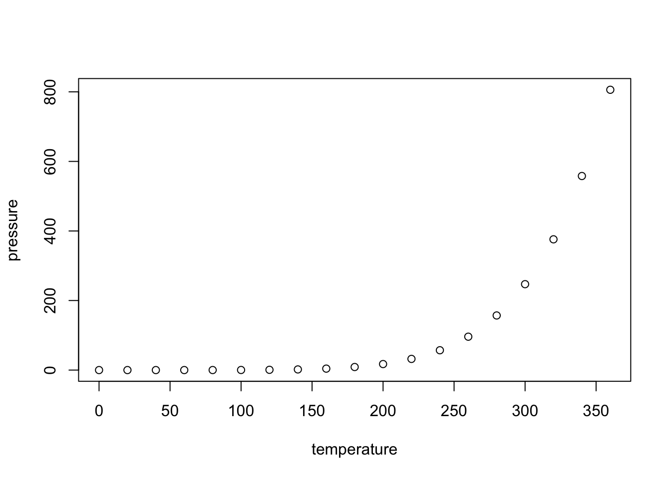
You can also embed plots, for example:

```{r, cache=TRUE}
summary(cars)
```

##      speed           dist       
##  Min.   : 4.0   Min.   :  2.00  
##  1st Qu.:12.0   1st Qu.: 26.00  
##  Median :15.0   Median : 36.00  
##  Mean   :15.4   Mean   : 42.98  
##  3rd Qu.:19.0   3rd Qu.: 56.00  
##  Max.   :25.0   Max.   :120.00

```{r, eval=FALSE}
# Need the knitr package to set chunk options
library(knitr)

# Set knitr options for knitting code into the report:
# - Don't print out code (echo)
# - Save results so that code blocks aren't re-run unless code changes (cache),
# _or_ a relevant earlier code block changed (autodep), but don't re-run if the
# only thing that changed was the comments (cache.comments)
# - show the error messages (message)
# - Don't clutter R output with warnings (warning)
# This _will_ leave error messages showing up in the knitted report
opts_chunk$set(echo=FALSE,
               cache=TRUE, autodep=TRUE, cache.comments=FALSE,
               message=TRUE, warning=FALSE)
```

References

1. Buckheit, J. B. & Donoho, D. L. Wavelab and reproducible research. (Stanford University, Standford CA 94305, USA, 1995).
2. Kühne, M. & Liehr, A. W. Improving the traditional information management in natural sciences. Data Sci. J. 8, 18–26 (2009).
3. the Yale Law School Roundtable on Data and Code Sharing. Reproducible research. Computing in Science Engineering 12, 8–13 (2010).
4. Wicherts, J. M. & Bakker, M. Publish (your data) or (let the data) perish! Why not publish your data too? Intelligence 40, 73–76 (2012).
5. Pasquier, T. et al. If these data could talk. Sci Data 4, 170114 (2017).
6. Peng, R. D. Reproducible research in computational science. Science 334, 1226–1227 (2011).
In the 1970s, the great computer scientist Donald Knuth wrote a mark-up language, and a rendering program for that language, called
TeX(pronounced “tech”), for writing complex mathematical documents. In the 1980s, the computer scientist Leslie Lamport extendedTeXin ways that made it rather more user-friendly, and called the resultLaTeX(pronounced “la-tech”)↩