Chapter 11 Applied thermochemistry: acid-base equilibria

Chapter summary:

• An acid is a molecule which can donate a hydrogen ion H⁺ and a base is an element that can accept a H⁺
• The level of pH dictates which of the conjugate acid and base forms are preponderant in a solution
• Reversely, pH is also dependent upon the concentrations of elements in a solution
• Graphical methods are very useful methods to visualize concentrations and to calculate pH
• The differences in orders of magnitude in concentrations allow to make very useful approximations in chemistry to calculate preponderant concentrations as well as the pH of solutions

11.1 The Brønsted–Lowry acid–base theory

According to the Brønsted-Lowry theory, an acid is any species that is capable of donating a hydrogen ion H⁺, and a base is any species capable of accepting a hydrogen ion, which requires a lone pair of electrons to bond to the H⁺ (Wikipedia_contributors2018-fr?). An acid necessarily contains an atom of hydrogen. The two forms exchanging a hydrogen ion a referred to as conjugate acid and base.

Technically, a proton or hydrogen ion cannot exist unhydrated in water solution. And technically, in water, a hydrogen ion is hydrated to produce the hydronium ion:

\[\begin{equation} H_2O + hydrogen \space ion \rightleftharpoons H_3O^+ \hspace{2.5cm} K_0 \tag{11.1} \end{equation}\]

So technically, donating a hydrogen ion for an acid necessarily involves the molecule of water as in the equilibrium (11.2)

\[\begin{equation} acid + H_2O \rightleftharpoons H_3O^+ + conjugate \: base \hspace{2.5cm} K_1 \tag{11.2} \end{equation}\]

One can dissociate, however this reaction in two elementary reactions as

\[\begin{equation} acid \rightleftharpoons hydrogen \space ion + conjugate \: base \hspace{2.5cm} K_2 \\ H_2O + hydrogen \space ion \rightleftharpoons H_3O^+ \hspace{2.5cm} K_0 \tag{11.3} \end{equation}\]

Because the activity of water is essentially constant in dilute aqueous solutions, the hydration of the hydrogen ion can be ignored in defining acid-base equilibria (Stumm and Morgan 1996). The thermodynamic convention sets the standard free energy change ΔG° for reaction (11.1) equal to zero, or its rate constant K₀=1. So from now on, the molecule of water is purposely omitted in acid-base reactions herein, and the hydrated hydrogen ion is written as H⁺.

In the equilibrium (11.4) below, the acid is represented as HA. It can donate a hydrogen ion H⁺. The anion A^- is referred to as the conjugate base.

\[\begin{equation} HA \rightleftharpoons A^- + H^+ \hspace{2.5cm} K_A \tag{11.4} \end{equation}\]

Another example of an acid, is illustrated in equilibrium (11.5) where the acid is an anion (cation in the generic example below), and the conjugate base is an uncharged molecule.

\[\begin{equation} HA^+ \rightleftharpoons A + H^+ \tag{11.5} \end{equation}\]

Some molecules can be both an acid and a base: they are referred to as being amphoteric. Water is the most famous amphoteric molecule as it can donate a hydrogen ion to yield a hydroxide OH^-, or gain an electron to form the hydronium cation H₃O⁺ as illustrated in equilibria (11.6)

\[\begin{equation} H_2O \rightleftharpoons OH^- + H^+ \\ H_2O + H^+ \rightleftharpoons H_3O^+ \tag{11.6} \end{equation}\]

By convention, however, the acid conjugate is always placed on the left of the equilibria, and the conjugate base and the hydrogen ion H⁺ are placed on the right side of the equilibrium.

11.2 Acid-base equilibrium parameters

11.2.1 K_A

Like for all chemical reactions, it is possible to write down the equilibrium constant as the product of the activities of the products divided by the product of the activities of the reactants as in equation (11.7):

\[\begin{equation} K_A = \frac{\{A^-\}\{H^+\}}{\{HA\}} \tag{11.7} \end{equation}\]

where the activity of HA is written as \(\{HA\}\).

For natural waters, a very good approximation of an element chemical activities is its concentration and the expression of K_A can be expressed as in equation (11.8):

\[\begin{equation} K_A = \frac{[A^-][H^+]}{[HA]} \tag{11.8} \end{equation}\]

where, e.g., the concentration of HA can be written as \([HA]\).

11.2.2 pK_A

When the concentration of both conjugate acids and bases are equal in a solution, the expression of K_A in equation (11.8) is simplified into

\[\begin{equation} K_A = [H^+] \tag{11.9} \end{equation}\]

Taking the negative of the common logarithm (base 10) on both side yields:

\[\begin{equation} -log(K_A) = -log \left([H^+]\right) \tag{11.10} \end{equation}\]

The right side of equation (11.10) is the definition of the pH. By analogy, one can define a new term

\[\begin{equation} pK_A = -log(K_A) \tag{11.11} \end{equation}\]

which corresponds to the pH value at which the concentrations of the conjugate acid and base are equal.

11.3 Self-ionization of water

In all aqueous solutions, the following reaction (11.12), referred to as the autoprotolysis must be considered:

\[\begin{equation} H_2O + H_2O \rightleftharpoons OH^- + H_3O^+ \tag{11.12} \end{equation}\]

Since in dilute solution the activity of water \({ \{H_2O \} = 1}\) the equilibrium constant for equilibrium (11.12), often referred to as the ‘ion product’ or ‘ionic product’ of water can be written as:

\[\begin{equation} K_w = \{OH^-\} \{H_3O^+\} \equiv \{OH^-\} \{H^+\} \tag{11.13} \end{equation}\]

According to Stumm and Morgan (1996),

at 25°C, K_w = 1.008 × 10^-14 and the pH = 7.00 corresponds to the exact neutrality in pure water ([H⁺] = [OH^-])

Technically, K_w changes with temperature, according to equation (11.14) (Harned and Owen 1958)

\[\begin{equation} log K_w = \frac{-4470.99}{T} + 6.0875 - 0.01706 T \tag{11.14} \end{equation}\]

With temperatures T expressed in °K. One can see in Figure 11.1 that the pH at exact neutrality varies with T°C reaching 7.37 at 5°C and decreasing down to about 6.84 at 35°C. So contrary to the common understanding that pH at neutrality is equal to 7, it actually changes with temperature, and not on an insignificant way. This is a reason why it is preferrable to calibrate pH probes using pH buffer solutions in the lab near 25°C. For all calculation purposes in this chapter, we will assume that the temperature is at 25°C, and we can therefore take that pH=7 at neutrality and that log K_w=-14.

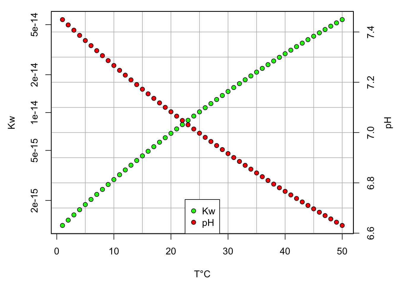
Figure 11.1: K_w and pH at exact neutrality as a function of T°C

11.4 Strong vs. weak acids

The concept of ionization of water defines the limits within which water activity remains equal to one, while the hydroxyde OH^- and hydronium H₃O⁺ or simpler hydrogen ion H⁺ coexist. At pH=0, all the ionization is in the form of H⁺, and conversely, at pH=14, all the autoprololysis of water yields only OH^-. Beyond these limits, i.e., pH less than 0 and greater than 14, one cannot consider these dilute solutions in water anymore.

So all acids for which the pK_A (i.e., -log(K_A)) is beyond the 0 to 14 values, are considered strong acids or strong bases. This means that in dilute solutions, the acid (or the base) can be considered entirely dissociated into its conjugate base (or acid). To better understand this, let us take nitric acid for which the pK_A=-1.4. This means that there is as much HNO₃ as there is NO₃^- at pH=-1.4. So for dilute solutions, we can consider that all HNO₃ has been dissociated into NO₃^-, and that in fact there is no measurable HNO₃ in solution.

Conversely, all other acids for which the pK_A is within 0 and 14 are considered weak acids, because depending on the pH, they can either be in the HA or A^- forms, if we take our generic equilibrium example (11.4). It turns out that many inorganic nutrients of interest and all organic acids are weak acids. This property makes them undergo transformations depending on the controlling pH, but also makes them play a very significant role in buffering the ambient pH. These weak acids are in large part responsible for the relative narrow range of pH in natural waters included in most cases between 4.5 and 8.5.

11.5 Mono- and polyprotic acids mole fractions

The first equilibrium (11.4) illustrates the case of a monoprotic acid, i.e., that can donate only one hydrogen ion. For our purposes, important monoprotic acids include \(HSO_4^{2-}\) and \(NH_4^+\). Among the inorganic nutrients important to environmental and ecological engineering, several are polyprotic acids, namely, phosphates, carbonates, and hydrogen sulfides. Polyprotic acids are acids that can donate more than one hydrogen ion. Because they have the ability to donate or gain a hydrogen ion, these polyprotic acids, with other species, play a very special role in buffering the pH of streams, ground, lake, and sea waters, as well as that of soil pore water.

The mono- and polyprotic acids mentioned above can take several forms, depending on the pH. Reversely, some of the biogeochemical processes at play, e.g., in streams or a wetland soil, will tend to add or remove some of the conjugate forms, possibly modifying the local pH over time. An important tool to understand the role played by environmentally important weak acids is to calculate the relative molar fraction of each of the conjugate forms as a function of pH. In the following, we will illustrate how to calculate the molar fraction for an example triprotic acid, as well as in the general case of an acid able to donate n hydrogen ions. Results of the general case apply to the monoprotic acids as well.

11.5.1 Triprotic acid example

Let us take a generic triprotic acid able to donate up to three hydrogen ions. Three equilibrium reactions coexist in solution, in addition to the autoprotolysis of water (11.15). Before we start the calculations of the molar fractions, let us establish some simple methodological rules that greatly help solve many of chemistry problems. Always:

1. Write all the reaction equilibria at play and the corresponding equilibrium constants
2. list all the ionic and the non-ionic forms at play
3. Establish the electroneutrality of the solution by balancing the positive and negative charges of the ions at play
4. Establish the conservation of mass when possible

---

1. Equilibria at play:

\[\begin{equation} H_3A \rightleftharpoons H_2A^- + H^+ \hspace{2.5cm} K_1 = \frac{[H_2A^-][H^+]}{[H_3A]}\\ H_2A^- \rightleftharpoons HA^{2-} + H^+ \hspace{2.5cm} K_2 = \frac{[H_2A^-][H^+]}{[HA^{2-}]}\\ HA^{2-} \rightleftharpoons A^{3-} + H^+ \hspace{2.5cm} K_3 = \frac{[HA^{2-}][H^+]}{[A^{3-}]}\\ H_2O \rightleftharpoons OH^- + H^+ \hspace{2.5cm} K_w = [H^+][OH^-] \tag{11.15} \end{equation}\]

2. List of the ionic forms:
   • cations: \(H^+\)
   • anions: \(H_2A^-\), \(HA^{2-}\), \(A^{3-}\), \(OH^-\)
   • all other forms: \(H_3A\), \(H_2O\)

3. Electroneutrality of the solution:
   • \([H^+] = [H_2A^-] + 2\times[HA^{2-}] + 3\times[A^{3-}] + [OH^-]\)
   • The factor 2 before \(2\times[HA^{2-}]\) expresses the relative contribution of the concentration \([HA^{2-}]\) to the total negative charge. The same is true for \(3\times[A^{3-}]\).

4. Conservation of mass:
   • The summation of all the conjugate forms is often referred to as ‘total concentration’ or \(C_T\)
   • \(C_T = [H_3A] + [H_2A^-] + [HA^{2-}] + [A^{3-}]\)

---

After establishing the constraints of the system, it is possible to evaluate the relative abundance of each of the conjugate forms, i.e., the molar fraction or the ratio between concentrations of each form and \(C_T\), the total concentration of all the forms. To get there, let us first express each of the conjugate forms as a function of \([H_3A]\). Using the equations for the reaction constants, and combining the expressions of \(K_1\), \(K_2\), and \(K_3\) from (11.15), it is possible to obtain:

\[\begin{equation} [H_2A^-] = [H_3A] \frac{K_1}{[H^+]} \\ [HA^{2-}] = [H_3A] \frac{K_1K_2}{[H^+]^2} \\ [A^{3-}] = [H_3A] \frac{K_1K_2K_3}{[H^+]^3} \\ \tag{11.16} \end{equation}\]

Replacing the expressions of each conjugate forms in (11.16) above, the equation of the conservation of mass then becomes:

\[\begin{equation} C_T = [H_3A] \times \left( 1 + \frac{K_1}{[H^+]} + \frac{K_1K_2}{[H^+]^2} + \frac{K_1K_2K_3}{[H^+]^3}\right) \tag{11.17} \end{equation}\]

or

\[\begin{equation} C_T = [H_3A] \times \left( \frac{[H^+]^3 + K_1[H^+]^2 + K_1K_2[H^+] + K_1K_2K_3}{[H^+]^3}\right) \tag{11.18} \end{equation}\]

The molar fraction \(\alpha_0\) of the fully hydrogen ionated acid can be expressed as:

\[\begin{equation} \alpha_0 = \frac{[H_3A]}{C_T} \tag{11.19} \end{equation}\]

or

\[\begin{equation} \alpha_0 = \frac{[H^+]^3}{[H^+]^3 + K_1[H^+]^2 + K_1K_2[H^+] + K_1K_2K_3} \tag{11.20} \end{equation}\]

By analogy, and using the reaction constant equations, the other molar fractions can be expressed as:

\[\begin{equation} \alpha_1 = \frac{[H_2A^-]}{C_T} = \frac{K_1[H^+]^2}{[H^+]^3 + K_1[H^+]^2 + K_1K_2[H^+] + K_1K_2K_3} \tag{11.21} \end{equation}\]

\[\begin{equation} \alpha_2 = \frac{[HA^{2-}]}{C_T} = \frac{K_1K_2[H^+]}{[H^+]^3 + K_1[H^+]^2 + K_1K_2[H^+] + K_1K_2K_3} \tag{11.22} \end{equation}\]

\[\begin{equation} \alpha_3 = \frac{[A^{3-}]}{C_T} = \frac{K_1K_2K_3}{[H^+]^3 + K_1[H^+]^2 + K_1K_2[H^+] + K_1K_2K_3} \tag{11.23} \end{equation}\]

Notice that for all molar fractions, the denominator does not change, only the numerator does.

11.5.2 Generalized polyprotic acid mole fractions

The example above can be used to draw the general case of a polyprotic acid which can donate n hydrogen ions (including for n = 1). Using the same methodology as before :

---

1. Equilibria at play:

\[\begin{equation} H_nA \rightleftharpoons H_{n-1}A^- + H^+ \hspace{0.6cm} K_{a1} = \frac{[H_{n-1}A^-][H^+]}{[H_nA]} \hspace{0.6cm} [H_{n-1}A^-] = [H_nA] \frac {K_{a1}}{[H^+]}\\ H_{n-1}A^- \rightleftharpoons H_{n-2}A^{2-} + H^+ \hspace{0.6cm} K_{a2} = \frac{[H_{n-2}A^{2-}][H^+]}{[H_{n-1}A]} \hspace{0.6cm} [H_{n-2}A^-] = [H_nA] \frac {K_{a1}K_{a2}}{[H^+]^2}\\ \\ \vdots \hspace{6cm} \vdots \hspace{6cm} \vdots\\ \\ HA^{(n-1)-} \rightleftharpoons A^{n-} + H^+ \hspace{0.6cm} K_{an} = \frac{[A^{n-}][H^+]}{[HA^{(n-1)-}]} \hspace{0.6cm} [A^{n-}] = [H_nA] \frac {K_{a1}K_{a2} \ldots K_{an}}{[H^+]^n}\\ \tag{11.24} \end{equation}\]

2. List of the ionic forms:
   • cations: \(H^+\)
   • anions: \(H_{n-1}A^-\), \(H_{n-2}A^{2-}\), … , \(A^{n-}\), \(OH^-\)
   • all other forms: \(H_nA\), \(H_2O\)

3. Electroneutrality of the solution:
   • \([H^+] = [H_{n-1}A^-] + 2\times[H_{n-2}A^{2-}] \space + \space ... \space + \space n\times[A^{n-}] + [OH^-]\)

4. Conservation of mass:
   • The summation of all the conjugate forms is often referred to as ‘total concentration’ or \(C_T\)
   • \(C_T = [H_nA] + [H_{n-1}A^-] + ... + [A^{n-}]\)

---

The generalized equation for the mole fraction \(i\)

\[\begin{equation} \alpha_i = \frac{[H_{n-i}A^{(n-i)-}]}{C_T} \\ \\ \\ \alpha_i = \frac{K_{a1}K_{a2} \ldots K_{ai}[H^+]^{n-i}}{[H^+]^n + K_{a1}[H^+]^{n-1} + K_1K_2[H^+]^{n-2} + \dots + K_{a1}K_{a2}\dots K_{an}} \tag{11.25} \end{equation}\]

11.5.3 Graphical illustration of mole fractions of ecologically relevant weak acids

11.5.3.1 Mole fraction for ammonium/ammonia

Now that we have defined the expressions for the molar fraction of weak acids, it is time to apply the generalized equation (11.25) to ecologically relevant weak acids. Let us start with ammonium \(NH_4^+\) and its conjugate base \(NH_3\). At 25°C, the pK_A is 9.28, or at pH = 9.28, \([NH_4^+] = [NH_3]\). At pH less than pK_A, \(NH_4^+\) is the preponderant form, and at pH greater than pK_A, \(NH_3\) becomes the preponderant form. One can see in Figure 11.2, that at pH less than 8, the molar fraction of ammonia is less than 5% of the total \([NH_4^+] + [NH_3]\) (sometimes referred to as Total Amoniacal Nitrogen, or TAN). For this reason, in most natural waters, \([NH_4^+]\) is by far the most preponderant form. Because in most natural waters, the concentrations of \(NH_4^+\) is relatively low (~< 0.2 mg N/L), there is very little loss of ammonia through volatilization. However, in animal waste water such as hog lagoons as they exist in North Carolina, ammonia volatilization is important. The pH of these lagoons range from 6.5 to 8.5 for an average of 7.8 (Barker, Zublena, and Walls 1994), yielding 3% of the TAN as ammonia. However, the total TAN concentration can easily reach 1000 to 2000 mg N/L, resulting in \([NH_3]\) between 30 and 60 mg N/L. The potential for ammonia volatilization is thus very high and occurs despite low molar fractions.

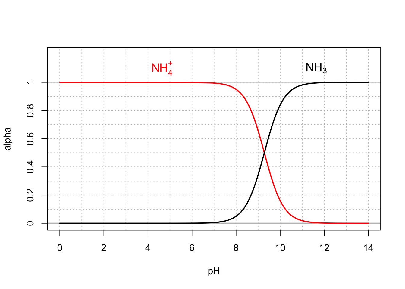
Figure 11.2: Molar fraction for ammonium and ammonia in dilute solutions at 25°C

Now, technically an important piece of information should have been added for the ammonium/ammonia molar fraction graph. Because ammonia is a gas that can equilibrate with the atmosphere, and is therefore an open system, the graph illustrated in Figure 11.2 corresponds to the case of a ‘closed system’, and in particular a system not directly open to the atmosphere. In reality, because of the pH range in natural waters, and the fact that ammonium is by far the most preponderant form, even when open to the atmosphere, the ammonium/ammonia equilibrium behaves very much like a closed system, in the case of low total ammoniacal concentrations.

11.5.3.2 Mole fraction for phosphate and its conjugated acids

The phosphate anion (\(PO_4^{3-}\)) has three conjugate acids, and is the dehydrogen ionated form of the triprotic phosphoric acid. The pK_A of the conjugate forms are at 25°C 2.12, 7.21, and 12.67. The preponderant forms present at pH between 4.5 and 8.5 are thus dihydrogen (\(H_2PO_4^-\)) and hydrogen (\(HPO_4^{2-}\)) phosphates (Figure 11.3). The byproduct of microbial respiration that finds its way into natural waters is thus rarely if ever \(PO_4^{3-}\) unlike presented in Chapter 8… The \(PO_4^{3-}\) form is still commonly used as a generic ‘phosphate’ molecule, regardless of pH considerations.

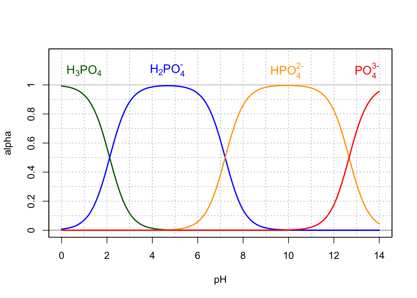
Figure 11.3: Molar fraction for the conjugate acid forms of the triprotic phosphoric acid in dilute solutions at 25°C

11.5.3.3 Mole fraction for sulfate and hydrogen sulfate

In most natural waters with pH between 4.5 and 8.5, sulfate is the preponderant form, and in the vast majority of cases, there is very little \(HSO_4^-\) (Figure 11.4). This figure also suggests that sulfuric acid (\(H_2SO_4^{2-}\)) does not exist in dilute waters in this form.

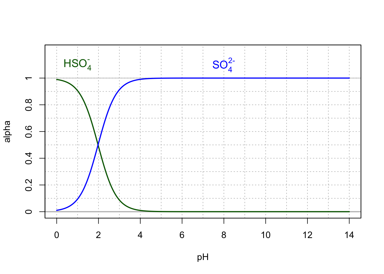
Figure 11.4: Molar fraction for the conjugate acid forms of the hydrogen sulfate and sulfate in dilute solutions at 25°C

11.5.3.4 Mole fraction of dissolved dihydrogen sulfide and conjugate bases

Now, for dihydrogen sulfide and carbon dioxide/carbonic acid, the volatile forms are present in very significant amounts for pH of natural waters. Because the molar fraction equation (11.25) only applies in closed systems, one might suggest that natural systems are in fact open systems, such that equation (11.25) just should not be used. True for open waters. However, there are lots of other ‘captive’ waters such as groundwater or sediment porewater, that are not directly open to the atmosphere and for which it is possible to use the molar fraction equation (11.25).

The pKa of the dihydrogen sulfide/hydrogen sulfide is 7.02 at 25°C, and there is still about 10% of \(H_2S_(aq)\) at pH=8 (Figure 11.5). The sulfide ion \(S^{2-}\), for most natural waters is not present and for the normal range of pH of natural waters, the two significant forms are \(H_2S_(aq)\) and \(HS^-\). There are consequences on bubble formation or gas ebullition in aquatic sediments as we shall see herein.

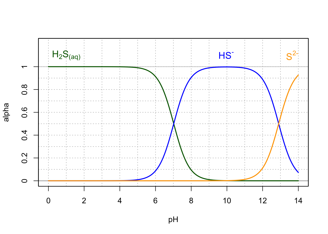
Figure 11.5: Molar fraction for the conjugate acid forms of the hydrogen sulfide in dilute solutions at 25°C

11.5.3.5 Mole fraction of hydrated carbon dioxide and carbonates

Similarly to the hydrogen sulfide diprotic acid, carbon dioxide in water can become hydrated and becomes the diprotic carbonic acid, which can donate up to two electrons. For the normal range of pH of natural waters, the two significant forms are \(H_2CO_3^o\) and \(HCO_3^-\) (Figure 11.6), where

\[\begin{equation} \{H_2CO_3^o\} = \{CO_{2(aq)}\} + \{H_2CO_3\}\\ \tag{11.26} \end{equation}\]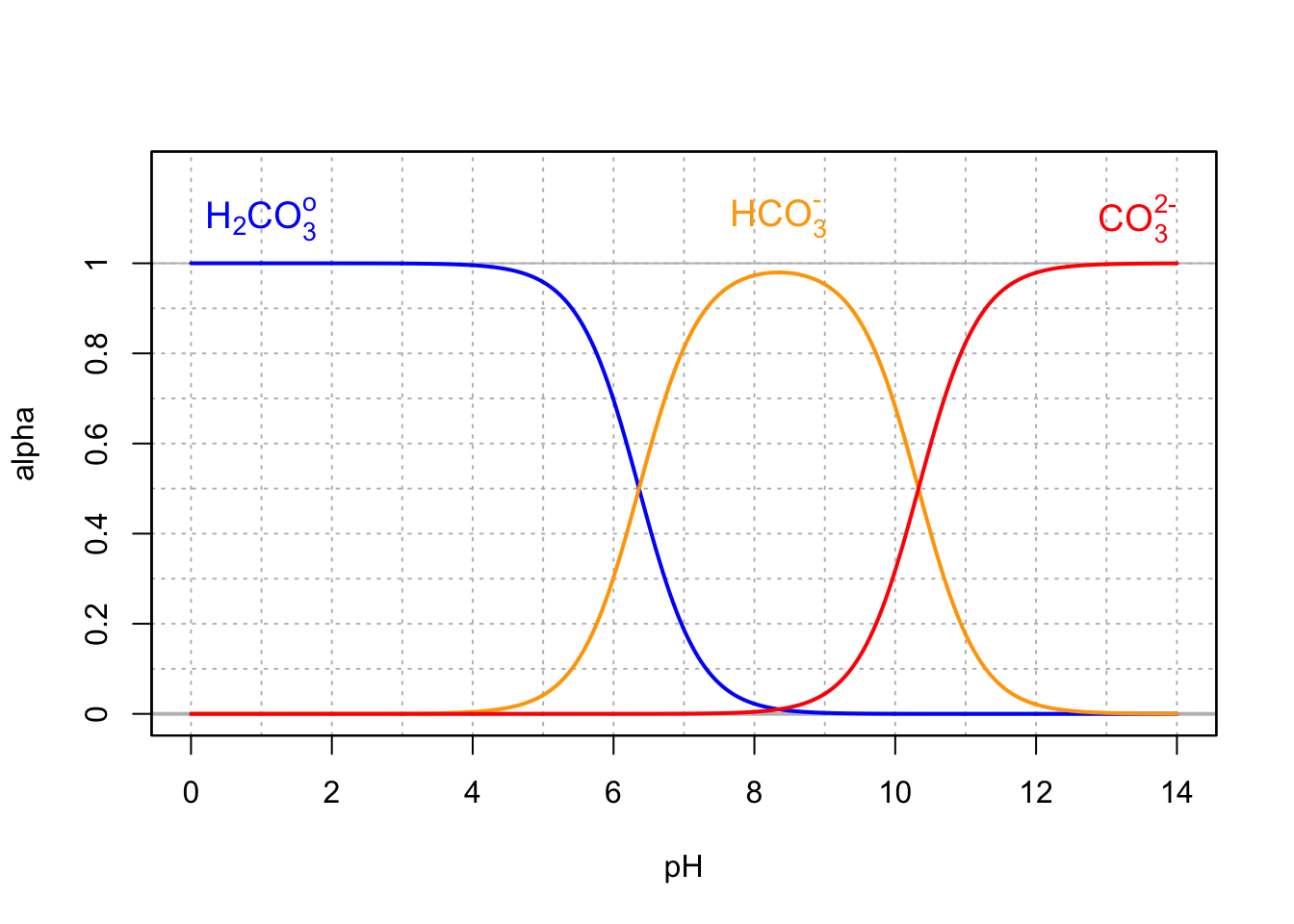

Figure 11.6: Molar fraction for the conjugate acid forms of the hydrated carbon dioxide, bicarbonate, and carbonate in dilute solutions at 25°C

The reason for combining \(CO_{2(aq)}\) and the true carbonic acid \(H_2CO_3\) into one composite \(H_2CO_3^o\) is to make apparent the diprotic nature of the carbonate system, i.e., it makes the protolysis of \(H_2CO_3^o\) more apparent considering the three species \(H_2CO_3^o\), \(HCO_3^{-}\), and \(CO_3^{2-}\) as in the equilibria below (equation (11.27)):

\[\begin{equation} H_2CO_3^o \rightleftharpoons HCO_3^- + H^+ \\ HCO_3^- \rightleftharpoons CO_3^{2-} + H^+ \tag{11.27} \end{equation}\]

But why not using carbonic acid proper (\(H_2CO_3\)) rather than this composite \(H_2CO_3^o\)? It is because the hydration of dissolved carbon dioxide into carbonic acid (equation (11.28)) occurs but the equilibrium is skewed towards the left with less than 0.3% of the carbon dioxide hydrated into \([H_2CO_3]\) (equilibrium constant K - equation (11.28) - values range from 350 to 990, with 650 commonly used (Stumm and Morgan 1996)).

\[\begin{equation} CO_{2(aq)} + H_2O \rightleftharpoons H_2CO_3 \hspace{3.5cm} K = \frac{\{CO_{2(aq)}\}}{\{H_2CO_3\}}\\ \tag{11.28} \end{equation}\]

The composite \(H_2CO_3^o\) is thus a notation to remind student chemists that in reality, there is relatively little carbonic acid in solution, and although \(CO_{2(aq)}\) would better represent the actual species in water, protolysis is only apparent from a hydrated \(CO_{2(aq)}\). One might wonder then how \(CO_{2(aq)}\) dissociates into \(HCO_3^{-}\)… It does not, the true carbonic acid \(H_2CO_3\) is the one that undergoes protolysis (i.e., the release of a hydrogen ion).

The kinetics of the series of reactions illustrated in equation (11.29) show that the limiting reaction is the hydration of the \(CO_{2(aq)}\) into \(H_2CO_3\), but that the overall effective hydration equilibrium from \(CO_{2(aq)}\) into \(HCO_3^-\) takes no more than a few minutes to establish (Stumm and Morgan 1996).

\[\begin{equation} CO_{2(aq)} + H_2O \hspace{0.5cm} \underset{fast}{\stackrel{slow}{\rightleftharpoons}} \hspace{0.5cm} H_2CO_3 \underset{}{\stackrel{very fast}{\rightleftharpoons}} H^+ + HCO_3^{-} \\ \tag{11.29} \end{equation}\]

Several byproducts of respiratory processes are gases: \(CO_2\), \(N_2\), \(N_2O\), \(H_2S\) and \(CH_4\). One of the consequences on wetland sediment porewater chemistry, is that the pH being relatively acidic, most of the inorganic sulfur and carbon byproduct of respiration are in the \(H_2S_{(aq)}\) form and \(CO_{2(aq)}\), rather than in their conjugate bases. For a given dissolved gas concentration, there corresponds, at equilibrium, an equivalent partial pressure in the gas phase above that water. The two are related by the Henry’s law (Henry and Banks 1803) that essentially says that the quantity of an ideal gas that dissolves in a definite volume of liquid is directly proportional to the pressure of the gas above it. This applying to all gases that might be dissolved in water (list above plus \(O_2\) although not in anaerobic sediment) such that one can add all the corresponding partial pressures of all the gases. If the summation of the partial pressures of all the dissolved gases becomes greater than one atmosphere plus the height of the water column above, then the solubility of all the gases is exceeded, and gas bubbles form (more details in chapter 13 dedicated to dissolved gases).

11.5.3.6 Mole fraction of common polyprotic organic acids

Many weak acids are involved at the cellular level and participate in buffering the solution into which the organelles “bathe” in cells. These include di- and triprotic acids. Oxalic (Figure 11.7), malonic, succinic, and fumaric acids are C2, C3, and C4 diprotic acids with carboxyl groups located on the outer carbons.

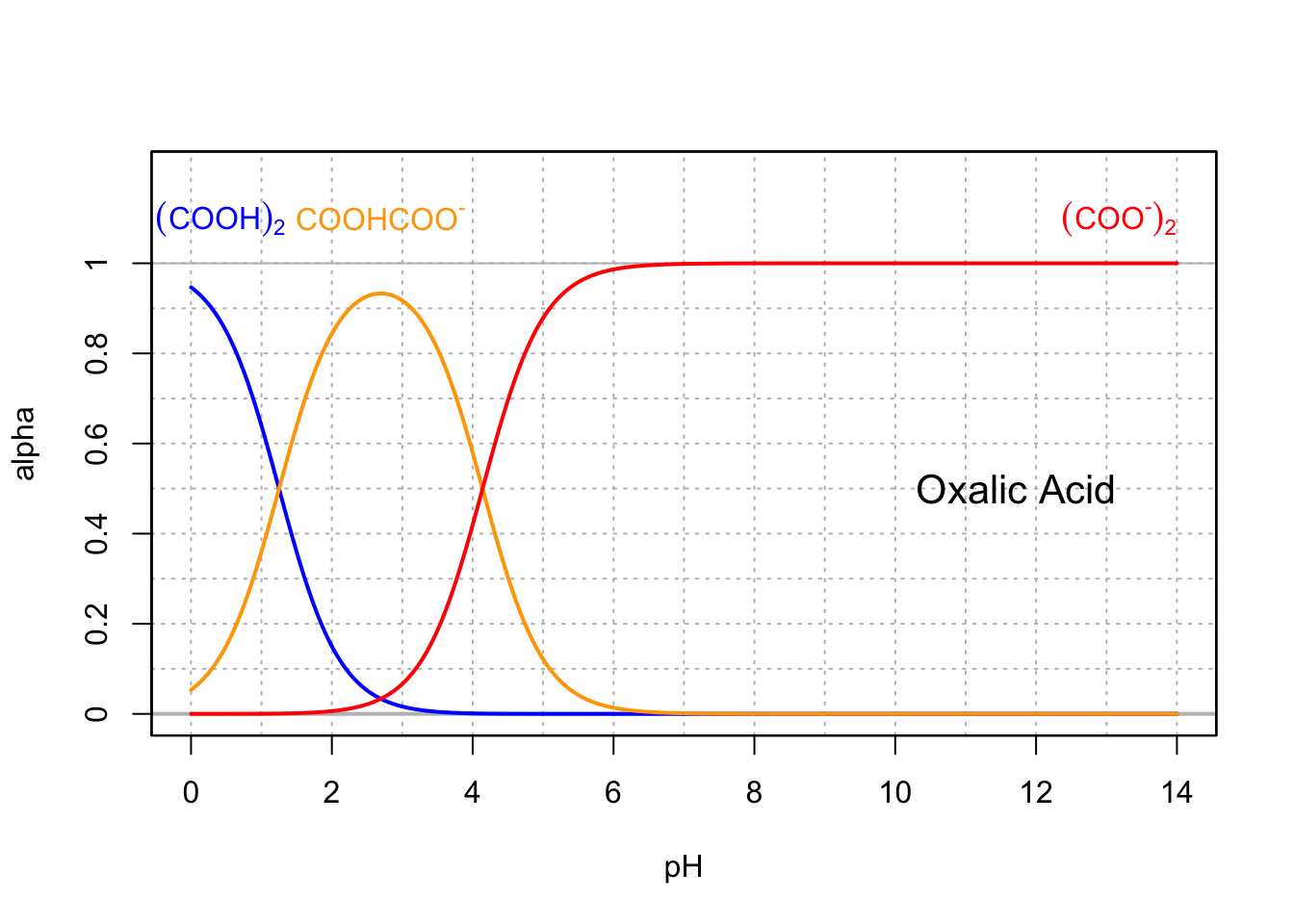
Figure 11.7: Molar fraction for the conjugate acid forms of the diprotic oxalic acid in dilute solutions at 25°C

Base conjugates are usually the preponderant forms at intracellular pH (7-7.4), so malonic (Figure 11.8), succinic (Figure 11.9), and fumaric (Figure 11.10) acids are thus usually referred to as malate, succinate, and fumarate, which are all involved in the citric acid cycle.

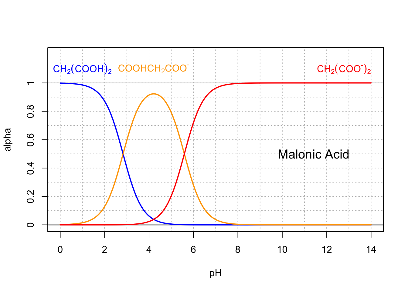
Figure 11.8: Molar fraction for the conjugate acid forms of the triprotic citric acid in dilute solutions at 25°C

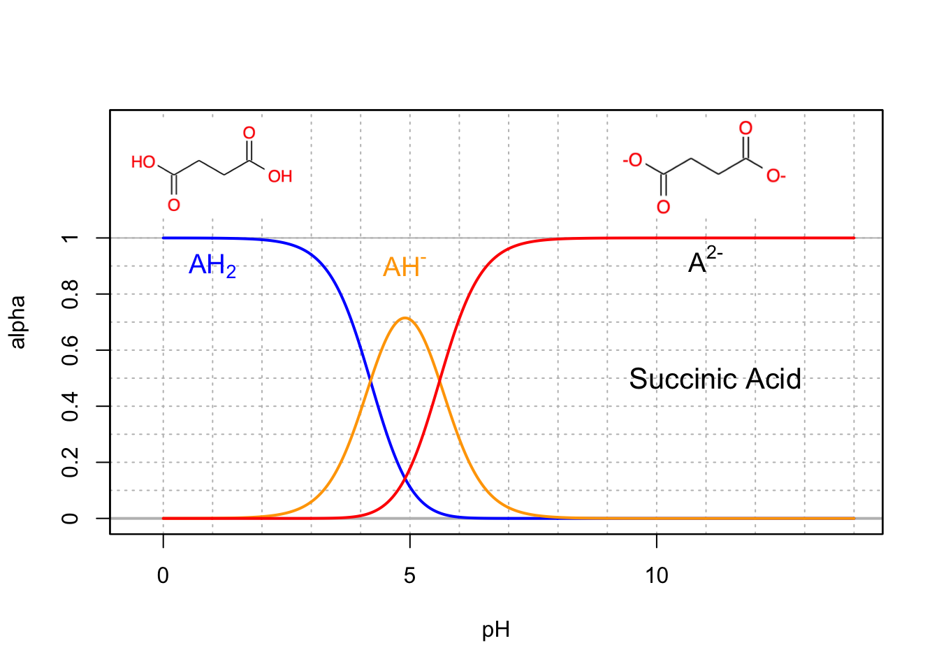
Figure 11.9: Molar fraction for the conjugate acid forms of the triprotic citric acid in dilute solutions at 25°C

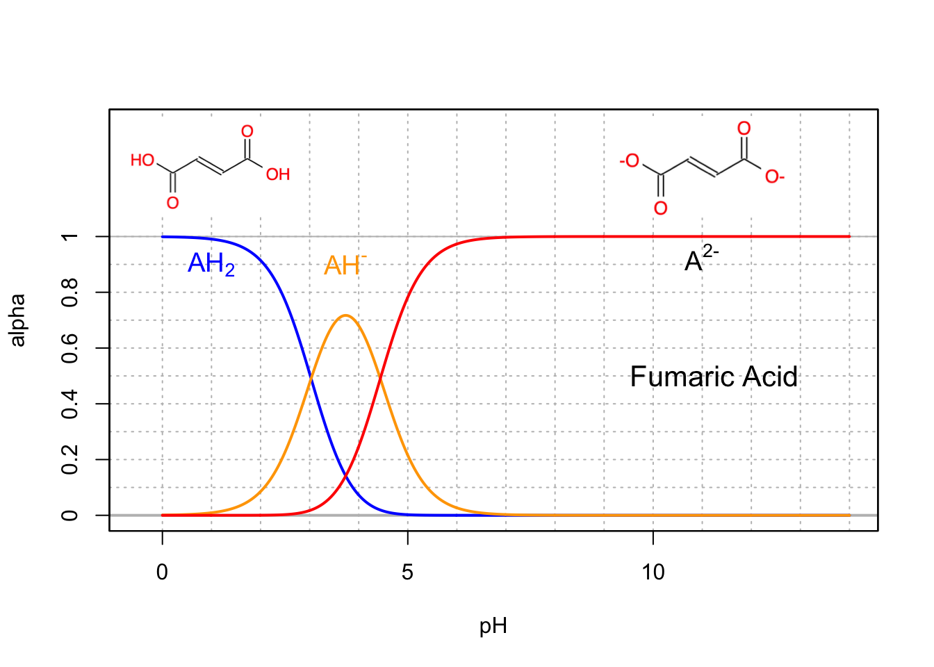
Figure 11.10: Molar fraction for the conjugate acid forms of the triprotic citric acid in dilute solutions at 25°C

In the last step of the citric acid, the oxalo-acetate (Figure 5.28) incorporates an acetate to form the triprotic citric acid (Figure 11.11), the molecule at the center of the citric acid cycle. All these acids do not seem to be able to provide that much buffering capacity for intracellular pH as they are all in their most basic conjugate form. However at pH 7, 20% of the citrate is in the AH^2- form.

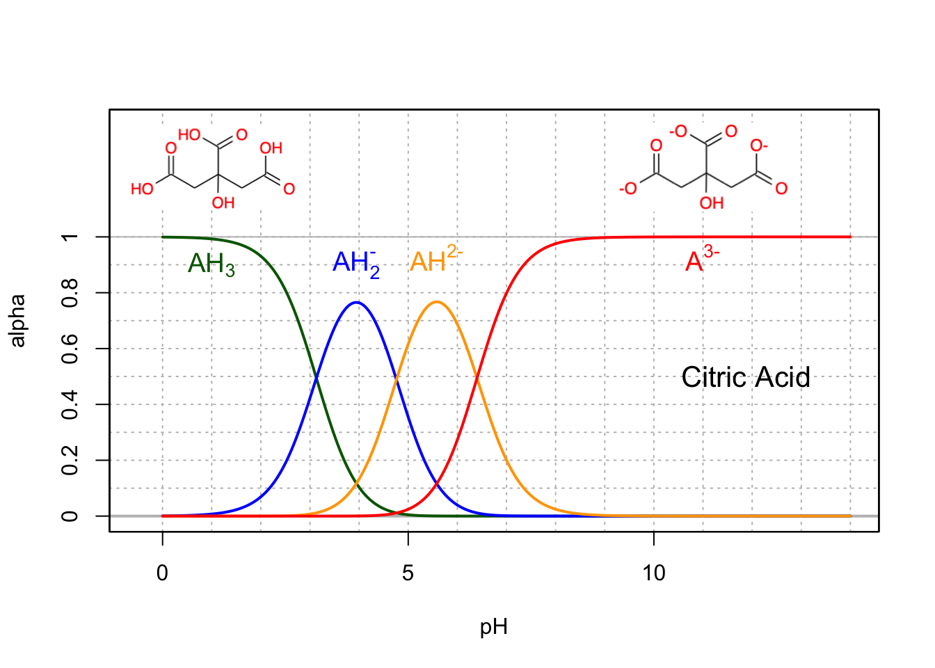
Figure 11.11: Molar fraction for the conjugate acid forms of the triprotic citric acid in dilute solutions at 25°C

Another interesting example of a potential triprotic acid is uric acid (Figure 11.12). Actually, it is somewhat surprising that it would behave as an acid at all, as it does not contain any carboxylic acid. However, the hydroxyl of the imidazol moeity does lose a hydrogen ion, but the other hydroxyl groups do not. In reality, uric acid does not behave like a polyprotic acid, but as a monoprotic acid…

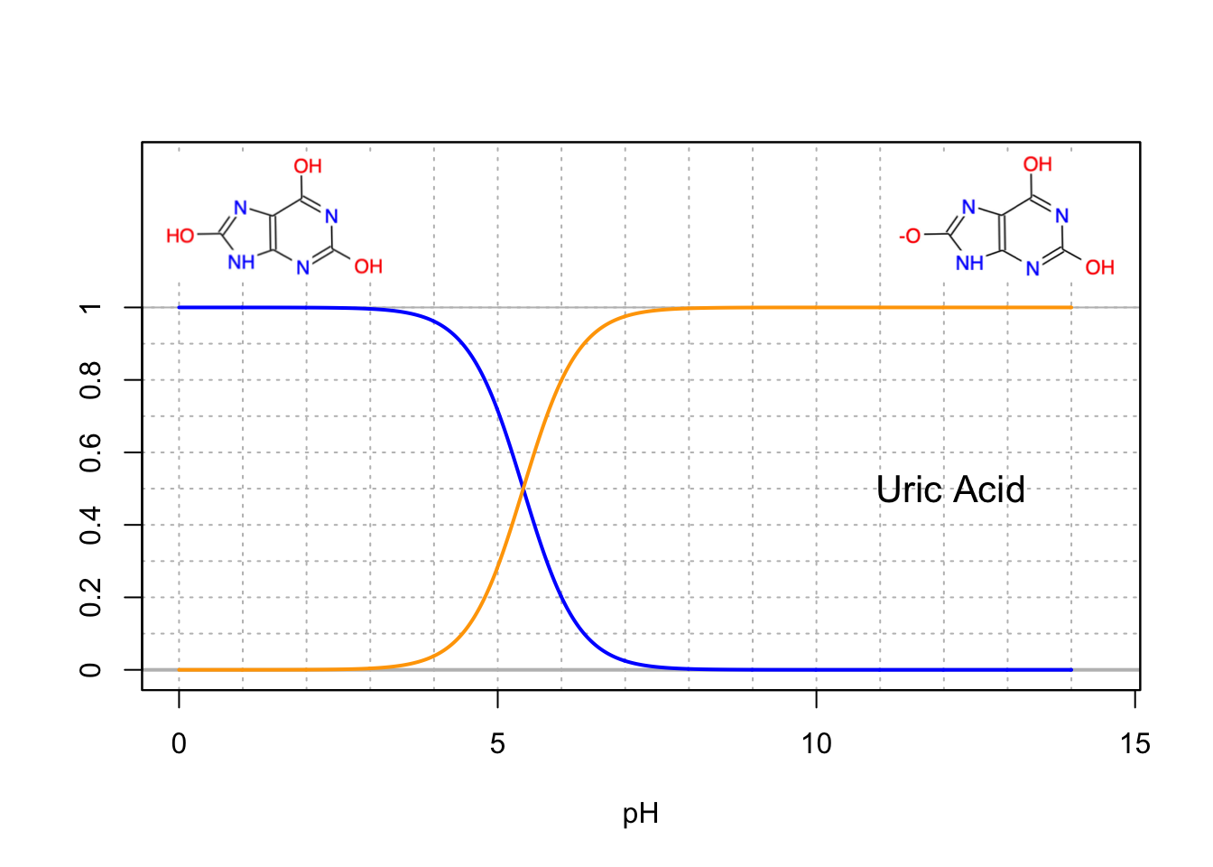
Figure 11.12: Molar fraction for the conjugate acid forms of the diprotic uric acid in dilute solutions at 25°C

Uric acid is a product of the metabolic breakdown of purine nucleotides, and is normally found in urine. Uric acid further decomposes in urea and a C3 molecule. The curious in you will write the Lewis dot structure and realize that the carbon in urea has zero electrons for itself, and so is the case for two of the carbons on uric acid, although it is an organic molecule! This means that all the energy has been squeezed out, which is not too surprising for a molecule that essentially is a waste product.

11.6 Equilibrium calculations using a graphical method

The graphical representation of the molar fraction highlights well the clear preponderant form for a given pH range, and the relative percentage of several forms for other pH values. Molar fractions are also independent of the total concentration. When the molar fractions are less than 1%, this method gives little graphical information on the relative abundance of the forms at play as the lines overlap each other.

Because the variation of pH represents variations of orders of magnitude in the hydrated hydrogen ion concentrations, the concentrations of conjugate forms can vary by orders of magnitude as a function of pH. The representation of the \(log(conc) = f(pH)\) opens the opportunity to graphically represent concentrations as a function of pH. As it turns out, this method can then be used to calculate pH values of a solution that would have been made from the addition of a salt.

11.6.1 Logarithm of concentrations as a function of pH

For this, let us first consider the theoretical salt AHCl added to one liter of water, which fully dissociates into \(AH^+ + Cl^-\), with \(AH^+\) being a weak acid. The goal of this exercise is to be able to graphically represent \(log(conc) = f(pH)\) for both conjugate forms \(AH^+\) and \(A\). For this, let us use the systematic method previously presented.

---

1. Equilibria at play:

\[\begin{equation} AH^+ \rightleftharpoons A + H^+ \hspace{2.5cm} K_A = \frac{[A][H^+]}{[AH^+]}\\ \tag{11.30} \end{equation}\]

2. List of the ionic forms:
   • cations: \(H^+\), \(AH^+\)
   • anions: \(OH^-\), \(Cl^-\)
   • all other forms: \(A\), \(H_2O\)

3. Electroneutrality of the solution:
   • \([H^+] + [AH^+] = [Cl^-] + [OH^-]\)

4. Conservation of mass:
   • \(C_T = [AH^+] + [A]\)

---

Using the conservation of mass equation, one can write:

\[\begin{equation} C_T = [AH^+] \times \left( 1 + \frac{K_A}{[H^+]} \right) \tag{11.31} \end{equation}\]

or

\[\begin{equation} C_T = [AH^+] \times \left( \frac{K_A + [H^+]}{[H^+]} \right) \tag{11.32} \end{equation}\]

This yields to the expression of both \([AH^+]\) and \([A]\):

\[\begin{equation} [AH^+] = \frac{C_T. [H^+]}{K_A + [H^+]} \\ [A] = \frac{C_T. K_A}{K_A + [H^+]} \tag{11.33} \end{equation}\]

The denominator of the expressions of \([AH^+]\) and \([A]\) is a summation, which does not go very well with the use of logarithms. Using XXI^st century technology, this really is not a problem and one can plot \(log(conc) = f(pH)\) with ease. But at the time when people were using slide rules, this was not so easy. The point is not to go back in time, but rather reflect on what it is that these expressions are telling and this involves the understanding of the physical meaning of what the equations represent.

Again, the goal here is to get a better representation of how the concentrations change as a function of pH. In the denominator \(K_A + [H^+]\), the \([H^+]\) varies on a logarithm scale as pH increases since \([H^+] = 10^{-pH}\). As a result, \([H^+]\) can increase or decrease very rapidly as a function of pH. The denominator can thus but dominated by either \(K_A\) or \([H^+]\). This means that in some cases, the summation in the denominator might be simplified by one of the two terms. The next step consists in defining for what pH values these conditions would be met.

---

• Case number 1: \([H^+] \gg K_A\)

For chemists, such a condition is traditionally approximated when \(K_A > 10 \times [H^+]\).

A series of equations ensues:

\[\begin{equation} [H^+] > 10 \times K_A \\ log([H^+]) > log(10) + log(K_A) \\ -log([H^+]) < -log(10) - log(K_A) \\ \tag{11.34} \end{equation}\]

or when

\[\begin{equation} pH < pK_A - 1 \tag{11.35} \end{equation}\]

So in this case, one can simplify the expressions of \([AH^+]\) and \([A]\) by:

\[\begin{equation} [AH^+] \approx C_T \hspace{3.5cm} [A] \approx \frac{C_T. K_A}{[H^+]} \\ \tag{11.36} \end{equation}\]

---

• Case number 2: \(K_A \gg [H^+]\)

This condition is approximated when \(K_A > 10 \times [H^+]\).

A series of equations ensues:

\[\begin{equation} K_A > 10 \times [H^+] \\ log(K_A) > log(10) + log([H^+]) \\ - log(K_A) < -1 - log([H^+]) \\ \tag{11.37} \end{equation}\]

or when

\[\begin{equation} pH > pK_A + 1 \tag{11.38} \end{equation}\]

So in this case, one can simplify the expressions of \([AH^+]\) and \([A]\) by:

\[\begin{equation} [AH^+] \approx \frac{C_T. [H^+]}{K_A} \hspace{3.5cm} [A] \approx C_T \\ \tag{11.39} \end{equation}\]

---

• Case number 3: \([AH^+]=[A]\)

When the \([AH^+]\) and \([A]\) are equal, one can write:

\[\begin{equation} C_T = 2 \times [AH^+] \\ [AH^+]=[A]= \frac{C_T}{2}\\ \tag{11.40} \end{equation}\]

\[\begin{equation} K_A = [H^+] \\ pH = pK_A \tag{11.41} \end{equation}\]

---

Let us now summarize these findings and calculate the \(log(conc) = f(pH)\) in table 11.1. The expressions of \(log[AH^+]\) and \(log[A]\) have been purposely left as \(C^{st} - pH\) and \(C^{st} + pH\), respectively, with \(C^{st}\) standing for a constant value. This is to emphasize that one does not need to numerically calculate the value of the constants, as one has all needed information to make a robust graphical representation of \(log(conc) = f(pH)\).

Table 11.1: Summary of the expressions and approximated expressions of \(conc\), and \(log(conc)\) for a monoprotic acid as a function of pH for \(H^+\), \(OH^-\), \(AH^+\), and \(A\)

	pH < pKA - 1		pH = pKA		pH > pKA + 1
\([H^+]\)	\(10^{-pH}\)		\(10^{-pH}\)		\(10^{-pH}\)
\([OH^-]\)	\(10^{-14+pH}\)		\(10^{-14+pH}\)		\(10^{-14+pH}\)
\([AH^+]\)	\(C_T\)		\(\frac{C_T}{2}\)		\(\frac{C_T . [H^+]}{K_A}\)
\([A]\)	\(\frac{C_T . K_A}{[H^+]}\)		\(\frac{C_T}{2}\)		\(C_T\)
\(log[H^+]\)	\(-pH\)		\(-pH\)		\(-pH\)
\(log[OH^-]\)	\(-14+pH\)		\(-14+pH\)		\(-14+pH\)
\(log[AH^+]\)	\(log(C_T)\)		\(log(C_T) - log(2)\)		\(C^{st} - pH\)
\(log[A]\)	\(C^{st} + pH\)		\(log(C_T) - log(2)\)		\(log(C_T)\)

The expressions show that for \(pH<pK_A-1\) and \(pH>pK_A+1\), \(log[AH^+]\) and \(log[A]\) follow straight lines of slope -1, 0, or +1 as a function of pH. It is thus possible to draw linear asymptotic lines, litterally, which the \(log[AH^+]\) and \(log[A]\) lines should follow for \(pH<pK_A-1\) and \(pH>pK_A+1\). The actual \(log[AH^+]\) and \(log[A]\) lines would then deviate from the asymptotic lines for \(pK_A-1<pH<pK_A+1\) and crossing at \(logC_T - 0.3\) at \(pH=pK_A\).

An example graph of \(log(conc) = f(pH)\) is provided in Figure 11.13. This is generally referred to at the Bjerrum plot. The lines \(log[H^+] = -pH\) and \(log[OH^-] = -14+pH\) are first plotted (in grey in Figure 11.13). The next step is to draw the asymptotic lines (dotted lines in Figure 11.13). These appear as straight lines as a function of pH as their equations indicate (Table 11.1). In reality, it is possible to extend these lines up to pH=pK_A. Indeed asymptotic lines both intersect at \(log[AH^+]=C_T\) and \(log[A]=C_T\) at \(pH=pK_A\) (Figure 11.13). To draw these asymptotic lines, one needs to find this intersection and then draw either horizontal lines or lines with slopes of -1 or +1 as applicable. This is the reason why one does not need to know the numerical values of the \(C^{st}\) (constant) in the equations in Table 11.1. In reality, drawing the \(log[H^+]\) and \(log[OH^-]\) curves follows the same procedure. These two lines must meet at \(log(conc)=-7\) at \(pH=7\), and have slopes of -1 and +1, respectively.

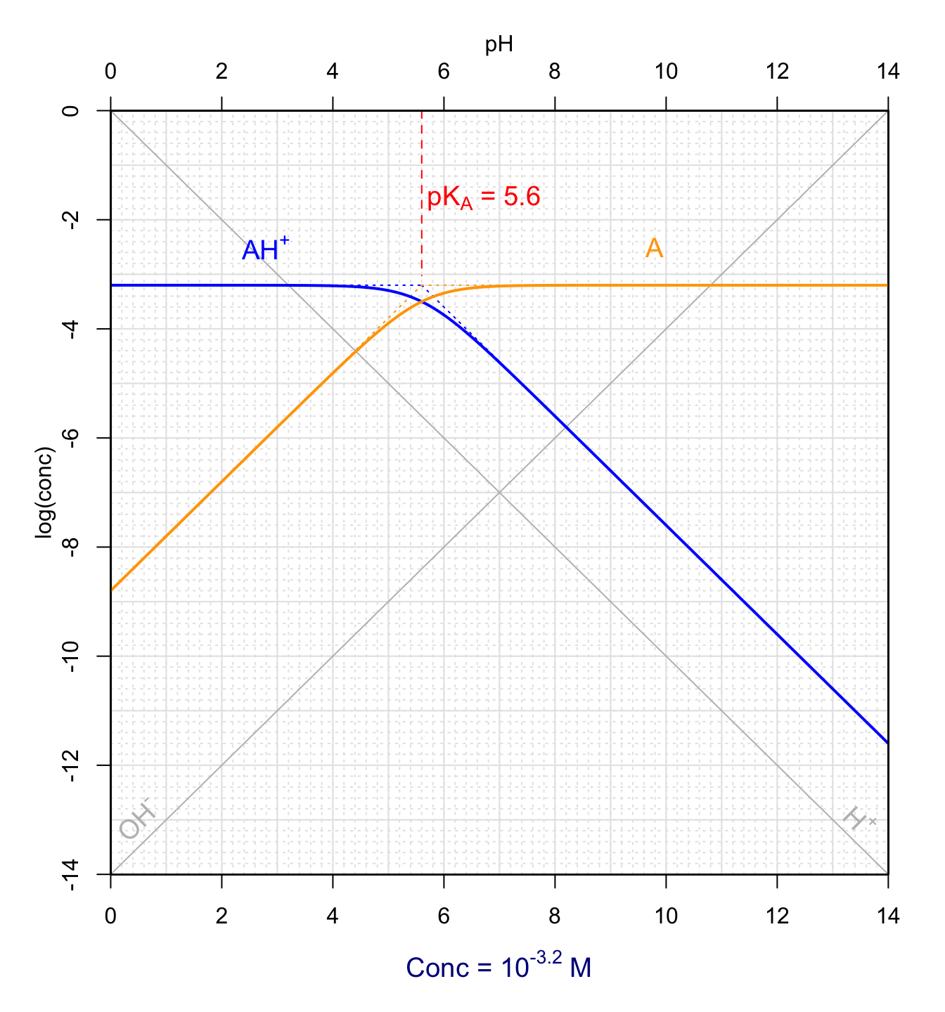
Figure 11.13: Forms of a hypothetical monoprotic acid for total concentration of 10^{-3.2}M as a function of pH at 25°C

The next step consists in superimposing the \(log[AH^+]\) and \(log[A]\) curves on the asymptotic lines outside of the \(pK_A \pm 1\) area. The next step consists in drawing the point where the two curves \(log[AH^+]\) and \(log[A]\) meet at \(pH=pK_A\), i.e., at \(log(C_T)-0.3\). Then one would manually connect the \(log[AH^+]\) and \(log[A]\) curves through the \(log(C_T)-0.3\) at \(pH=pK_A\) point, such as the tangent of the curves at \(pH=pK_A-1\) and \(pH=pK_A+1\) match the linear portions outside of the \(pK_A \pm 1\) area. Obviously for this book, the manual drawing of this curve cannot be achieved and the actual \(log(conc) = f(pH)\) have been plotted for \([AH^+]\) and \([A]\). One can observe that the actual curve apparently deviates from the asymptotic lines curves not at \(pK_A \pm 1\) but rather at \(pK_A \pm 1.4\).

11.6.2 Graphical approach to calculate pH for a monoprotic acid

The graphical approach illustrated in Figure 11.13 gives a nice way to quickly see whether some ion concentrations are much smaller than other, and whether one can assume some forms to be negligible compared to others.

So in the example above, combining the electroneutrality equation to that of the conversion of mass, and realizing that \([Cl^-]=C_T\) yields:

\[\begin{equation} [H^+] + [AH^+] = [Cl^-] + [OH^-] \\ [H^+] + [AH^+] = [AH^+] + [A] + [OH^-] \\ [H^+] = [A] + [OH^-] \tag{11.42} \end{equation}\]

So now, this is where it is important to be able to assess the physical reality of the \([A] + [OH^-]\) summation. It is easy to visualize on Figure 11.13 the relative importance of \([A]\) vs \([OH^-]\). In the figure, and for \(pH<pK_A\), \([OH^-] \leq 10^{-5} [A]\). One can safely assume that \([A] + [OH^-] \approx [A]\). Hence, in these cases, \([H^+] \approx [A]\), which means that pH can be graphically determined at the intersection between the \(log[H^+]\) and \(log[A]\) lines (Figure 11.14). The conditions for this graphical determination are that the \(log[A]\) curve be in its linear portion and that at the intersection, \([A]>10[OH^-]\). Figure 11.14 is an interactive graph where one can rapidly graphically determine pH as a function of variable \(pK_A\) and \(C_T\).

Figure 11.14: Graphical determination of pH as a function of variable pK_A and C_T for a hypothetical AHCl weak acid salt added into solution. Also available at this link

Now, the graphs in Figures 11.13 and 11.14 were derived for an \(AHCl\) hypothetical salt fully dissociating into \(AH^+\), \(A\) and \(Cl^-\). An analogous analysis can be derived for a weak base salt of formula \(ANa\) which would fully dissociate into \(HA\), \(A^-\) and \(Na^+\). In this case, the combination of the electroneutrality and conservation of mass would yield \([H^+] + [HA] = [OH^-]\). Using the same reasoning as before, pH can be graphically determined at the intersection between the \(log[OH^-]\) and \(log[HA]\) lines, and provided that the \(log[HA]\) curve be in its linear portion and that at the intersection \([HA]>10[H^+]\).

Figure 11.15: Graphical determination of pH as a function of variable pK_A and C_T for a hypothetical ANa weak base salt added into solution

Notice that when a hypothetical \(AHCl\) salt is added to solution, the pH tends to be acidic, and reversely, when a \(ANa\) salt is added, the pH tends to be basic. This is expected as the salts fully dissociate into, \(AH^+\) and \(Cl^-\), and \(A^-\) and \(Na^+\), in the first and second cases, respectively. In the first case, the initial form is thus the acid conjugate form \(AH^+\) which is first in solution, and that later dissociates into its conjugate base, thus releasing \(H^+\) and hence lowering the pH. In the second case, the conjugate base \(A^-\) is released in water first and consumes \(H^+\) to form its conjugate acid \(HA\), hence increasing the pH.

11.6.3 Graphical approach to calculate pH for a triprotic acid

Following the same procedure as that presented for a monoprotic acid, there are interesting points to highlight when plotting \(log(conc)=f(pH)\) for a triprotic acid. It turns out that phosphate triprotic base has a particular relevance for ecological engineering, so it is interesting to use phosphate as an illustration on how to derive \(log(conc) = f(pH)\) and graphically calculate pH for polyprotic acid/bases. Equation (11.17) derived above for a triprotic acid is:

\[\begin{equation} C_T = [H_3A] \times \left( 1 + \frac{K_1}{[H^+]} + \frac{K_1K_2}{[H^+]^2} + \frac{K_1K_2K_3}{[H^+]^3}\right) \tag{11.17} \end{equation}\]

For a monoprotic acid, the last two terms to the right did not exist, and it was relatively easy to express \([AH^+]\) and \([A]\) as in equation (11.33):

\[\begin{equation} [AH^+] = \frac{C_T. [H^+]}{K_A + [H^+]} \\ [A] = \frac{C_T. K_A}{K_A + [H^+]} \tag{11.33} \end{equation}\]

and then find the conditions for which the denominator could be simplified when \(K_A \gg [H^+]\) or \([H^+] \gg K_A\). But with the two extra terms in (11.17), this cannot be done as easily. The solution to this problem is, again, to realize the relative importance of the different terms in (11.17) and make simplifications and approximations that are amply sufficient to obtain robust graphical representations of the \(log(conc)=f(pH)\). Indeed, one can make the hypothesis that for pH near pK₁, \([H_3A]\) and \([H_2A^-]\) are by far the most prepoderant forms, such that the conservation of mass equation:

\[\begin{equation} C_T = [H_3A] + [H_2A^-] + [HA^{2-}] + [A^{3-}] \tag{11.43} \end{equation}\]

can be approximated into

\[\begin{equation} C_T \approx [H_3A] + [H_2A^-] \tag{11.44} \end{equation}\]

This is now a familiar problem which has already been solved for a monoprotic acid, for \(pH < pK_1 - 1\) and for \(pH > pK_1 + 1\) (Table 11.1). For example, for \(pH < pK_1 - 1\) and by analogy to results summarized in Table 11.1, all concentrations can be approximated by:

\[\begin{equation} [H_3A] \approx C_T \\ [H_2A^-] \approx \frac{C_T.K_1}{[H^+]} \\ [HA^{2-}] \approx \frac{C_T.K_1.K_2}{[H^+]^2} \\ [A^{3-}] \approx \frac{C_T.K_1.K_2.K_3}{[H^+]^3} \tag{11.45} \end{equation}\]

Obviously, the conservation of mass equation can be simplified the same way for pH near pK₂, where \([H_2A^-]\) and \([HA^{2-}]\) can be hypothesized to be largely preponderant, and similarly for pH near pK₃, where \([HA^{2-}]\) and \([A^{3-}]\) can be hypothesized to be preponderant. In the end, it is possible, for given pH ranges outside of the \(pK_x \pm 1\) to simplify the equations of each of the conjugate acid forms, and the expression of \(log(conc)=f(pH)\). For a triprotic acid, this is summarized in Table 11.2 below.

Table 11.2: Summary of the expressions and approximated expressions of \(conc\), and \(log(conc)\) for a triprotic acid as a function of pH for \(H^+\), \(OH^-\), \([H_3A]\), \([H_2A^-]\), \([HA^{2-}]\), and \([A^{3-}]\)

	pH < pK1-1		pK1+1< pH < pK2-1		pK2+1< pH < pK3-1		pH > pK3+1
\([H^+]\)	\(10^{-pH}\)		\(10^{-pH}\)		\(10^{-pH}\)		\(10^{-pH}\)
\([OH^-]\)	\(10^{-14+pH}\)		\(10^{-14+pH}\)		\(10^{-14+pH}\)		\(10^{-14+pH}\)
\([H_3A]\)	\(C_T\)		\(\frac{C_T.[H^+]}{K_1}\)		\(\frac{C_T.[H^+]^2}{K_1.K_2}\)		\(\frac{C_T.[H^+]^3}{K_1.K_2.K_3}\)
\([H_2A^-]\)	\(\frac{C_T.K_1}{[H^+]}\)		\(C_T\)		\(\frac{C_T.[H^+]}{K_2}\)		\(\frac{C_T.[H^+]^2}{K_2.K_3}\)
\([HA^{2-}]\)	\(\frac{C_T.K_1.K_2}{[H^+]^2}\)		\(\frac{C_T.K_2}{[H^+]}\)		\(C_T\)		\(\frac{C_T.[H^+]}{K_3}\)
\([A^{3-}]\)	\(\frac{C_T.K_1.K_2.K_3}{[H^+]^3}\)		\(\frac{C_T.K_2.K_3}{[H^+]^2}\)		\(\frac{C_T.K_3}{[H^+]}\)		\(C_T\)
\(log[H^+]\)	\(-pH\)		\(-pH\)		\(-pH\)		\(-pH\)
\(log[OH^-]\)	\(-14+pH\)		\(-14+pH\)		\(-14+pH\)		\(-14+pH\)
\(log[H_3A]\)	\(log(C_T)\)		\(C^{st} - pH\)		\(C^{st} - 2pH\)		\(C^{st} - 3pH\)
\(log[H_2A^-]\)	\(C^{st} + pH\)		\(log(C_T)\)		\(C^{st} - pH\)		\(C^{st} - 2pH\)
\(log[HA^{2-}]\)	\(C^{st} + 2pH\)		\(C^{st} + pH\)		\(log(C_T)\)		\(C^{st} - pH\)
\(log[A^{3-}]\)	\(C^{st} + 3pH\)		\(C^{st} + 2pH\)		\(C^{st} + pH\)		\(log(C_T)\)

Similarly to the case for monoprotic acids, the equations for the \(log(conc)=f(pH)\) in Table 11.2 are sometimes truncated into, e.g., \(C^{st} + pH\), \(C^{st}\) meaning ‘constant’. The reason for this is that these equations correspond to the equations of the straight lines that serve as asymptotic lines for the actual \(log(conc)\) curves. For sections with the slopes of ±1, these straight lines intersect at \(pK_x\). To draw the straight lines with the slopes of ±2, one may consider two facts:

• the linear sections with the slopes of ±2 intersect at \(\frac{pK_x+ pK_{x+1}}{2}\) for \(log(conc) = log(C_T)\) for x=1 and x=2 (not shown in Figure 11.16 for clarity reasons), or,
• the sections with the slopes of ±2 intersect the linear sections with the slopes ±1 at \(pK_x\) (shown in Figure 11.16).

It is thus possible to draw all these asymptotic lines as illustrated in Figure 11.16 below for the conjugate acids of phosphate \(PO_4^{3-}\). Following the principles described in section 11.6.2 above, the \(log(conc)\) curves follow the asymptotic lines outside the \(pH=pK_x \pm 1\). The actual curves illustrated in Figure 11.16 actually deviate from the asymptotic lines for \(pH=pK_x \pm 1.4\) as already observed in Figure 11.13. Again, this is of minor importance to graphically determine the pH of a solution.

One can also verify that for pH near pK_x, there are two preponderant forms, and that other forms are at least 10⁵ times lower, which justifies the approach used to simplify the equation of conservation of mass (equation (11.43)) to only two terms (e.g., equation (11.44)). Notice that the curves for the equations \(C^{st} \pm 3pH\) are off the chart and do not appear on Figure 11.16.

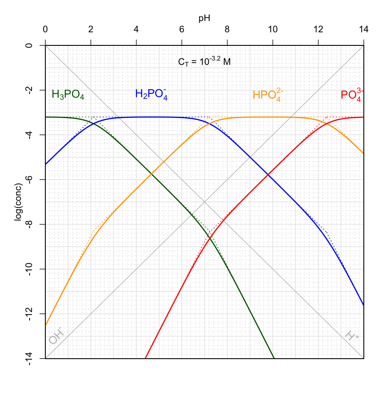
Figure 11.16: Forms of polyprotic phosphoric acid for total concentration of 10^-3.2M as a function of pH at 25°C. pK₁=2.12; pK₂=7.21; pK₃=12.37

With this graph in hand, and for \(C_T = 10^{-3.2}M\) as illustrated in Figure 11.16, it becomes possible to graphically evaluate the pH of a solution in which a weak acid salt, e.g., \(NaH_2PO_4\), or a weak base salt, e.g., \(CaHPO_4\) would be added in solution for a final \(C_T = 10^{-3.2}M\).

---

In the case of the \(NaH_2PO_4\) salt added, combining the electroneutrality and conservation of mass equations would yield:

\[\begin{equation} [H_3PO_4] + [H^+] = [HPO_4^{2-}] + 2 [PO_4^{3-}] + [OH^-] \tag{11.46} \end{equation}\]

One can seen on Figure 11.16 that for this \(C_T\), \([H_3PO_4] < 10[H^+]\), and \(2 [PO_4^{3-}] + [OH^-] \ll [HPO_4^{2-}]\), such that equation (11.46) can be approximated as \([H^+] \approx [HPO_4^{2-}]\). This means that the pH would correspond to that of the intersection between the \(log[H^+]\) and \(log[HPO_4^{2-}]\) lines.

---

In the case of \(CaHPO_4\) salt added, combining the electroneutrality and conservation of mass equations would yield:

\[\begin{equation} 2[H_3PO_4] + [H_2PO_4^-] + [H^+] = [PO_4^{3-}] + [OH^-] \tag{11.47} \end{equation}\]

One can seen on Figure 11.16 that for this \(C_T\), \(2[H_3PO_4] + [H^+] \ll [H_2PO_4^-]\), and that \([PO_4^{3-}] \ll [OH^-]\), such that equation (11.47) can be approximated as \([H_2PO_4^-] \approx [OH^-]\). This means that in this case the pH would correspond to that of the intersection between the \(log[H_2PO_4^-]\) and \(log[OH^-]\) lines.

---

Such pH determinations can be done for a variety of \(C_T\) values corresponding to the addition of the weak acid \(NaH_2PO_4\) salt, and to the addition of the weak base salt \(CaHPO_4\). Several conditions must be met, including that the simplifications described above apply, and that the curves cross on their linear portions. An illustration of the possibilities, or not, of graphically determining the pH is provided in Figure 11.17.

Figure 11.17: Graphical determination of pH as a function of variable C_T when the weak acid salt \(NaH_2PO_4\), and when the weak base salt \(CaHPO_4\) are added into solution

11.6.4 Dissolved CO₂ and carbonates in a closed system

Before this chapter, \(CO_2\) has been treated in this book as the waste product of respiration, and the entry level of the conversion of photonic energy into chemical energy. Carbon dioxide has additional major roles: in this chapter, we will introduce its impact on pH of surface and sediment waters.

There are four major ideas for which the equilibria involving \(CO_2\) and the carbonates matters:

1. Because all organotrophic respiratory processes produce \(CO_2\) as a waste product (see sections 8.2; summary Figure 8.15), the potential to have dissolved \(CO_2\) in surface and sediment water is high.
2. \(CO_2\) is a very soluble gas that readily dissolves in water (details in chapter 13; summary Figure 13.4).
3. Dissolved carbon dioxide reacts with water to theoretically form carbonic acid. However, the equilibrium is balanced towards \(CO_2\) rather than \(H_2CO_3\), and there is little actual carbonic acid in water. Its ability to release hydrogen ions (\(H^+\)) is not affected, however, and \(CO_2\) practically participate in releasing \(H^+\) and can be viewed as a diprotic acid (details in section 11.5.3.5 above).
4. Carbonate (\(CO_3^{2-}\)) reacts with cations such as \(Ca^{2+}\), \(Mg^{2+}\), \(Na^{+}\), \(K^+\), and \(Fe^{2+}\) to form carbonate rocks and minerals. Upon dissolution, these solids may add the conjugate base of the diprotic carbonic acid to the overall equilibria, and thus play a role in the pH of water.

In the case of a closed system, such as would be the case for sediment porewater, one may apply the general equations and concepts described above to the dissolved \(CO_2\) and carbonate equilibria. In section 11.5.3.5, we saw that in reality the hydration of \(CO_{2(aq)}\) into carbonic acid \(H_2CO_3\) is slow such that about 0.3% of \(CO_2\) gets hydrated into carbonic acid (Stumm and Morgan 1996). Howver, the deprotonation of carbonic acid is rather efficient (see equation (11.29)), such that it is customary to introduce the conceptual \(H_2CO_3^o\), which behaves like a diprotic acid:

\[\begin{equation} \{H_2CO_3^o\} = \{CO_{2(aq)}\} + \{H_2CO_3\}\\ \tag{11.26} \end{equation}\]

---

1. Equilibria at play:

\[\begin{equation} H_2CO_3^o \rightleftharpoons HCO_3^- + H^+ \hspace{2.5cm} K_{a1} = \frac{[HCO_3^-][H^+]}{[H_2CO_3^o]}\\ HCO_3^- \rightleftharpoons CO_3^{2-} + H^+ \hspace{2.5cm} K_{a2} = \frac{[CO_3^{2-}][H^+]}{[HCO_3^-]}\\ H_2O \rightleftharpoons OH^- + H^+ \hspace{2.5cm} K_{w} = [OH^-][H^+] \tag{11.48} \end{equation}\]

2. List of the chemical forms at play:
   • cations: \(H^+\)
   • anions: \(OH^-\), \(HCO_3^-\), \(CO_3^{2-}\)
   • all other forms: \(H_2CO_3^o\), \(H_2O\)

3. Electroneutrality of the solution:
   • \([H^+] = 2 \times [CO_3^{2-}] + [HCO_3^-] + [OH^-]\)

4. Conservation of mass (closed system):
   • \(DIC = [H_2CO_3^o] + [HCO_3^-] + [CO_3^{2-}]\)

In the case of carbonates and carbon dioxide, the \(C_T\) term previously used and standing for ‘total concentration’ is appropriately replaced by the term Dissolved Inorganic Carbon (DIC), as noted above. Remember that in \(DIC = [CO_{2(aq)}] + [H_2CO_3] + [HCO_3^-] + [CO_3^{2-}]\).

---

Applying the general terms derived in Table 11.2, the approximate terms for \([H_2CO_3^o]\), \([HCO_3^-]\), and \([CO_3^{2-}]\) can be expressed as a function of pH, DIC, \(K_{a1}\), and \(K_{a2}\) in Table 11.3 below. The log(conc) terms are plotted as a function of pH on the Bjerrum plot below in Figure 11.18 below

Table 11.3: Summary of the expressions and approximated expressions of \(conc\), and \(log(conc)\) for the diprotic acid \([H_2CO_3^o]\) (practically dissolved \(CO_2\)) as a function of pH for \(H^+\), \(OH^-\), \([H_2CO_3^o]\), \([HCO_3^-]\), and \([CO_3^{2-}]\)

	pH < pKa1-1		pKa1+1< pH < pKa2-1		pH > pKa2+1
\([H^+]\)	\(10^{-pH}\)		\(10^{-pH}\)		\(10^{-pH}\)
\([OH^-]\)	\(10^{-14+pH}\)		\(10^{-14+pH}\)		\(10^{-14+pH}\)
\([H_2CO_3^o]\)	\(DIC\)		\(\frac{DIC.[H^+]}{K_{a1}}\)		\(\frac{DIC.[H^+]^2}{K_{a1}.K_{a2}}\)
\([HCO_3^-]\)	\(\frac{DIC.K_{a1}}{[H^+]}\)		\(DIC\)		\(\frac{DIC.[H^+]}{K_{a2}}\)
\([CO_3^{2-}]\)	\(\frac{DIC.K_{a1}.K_{a2}}{[H^+]^2}\)		\(\frac{DIC.K_{a2}}{[H^+]}\)		\(DIC\)
\(log[H^+]\)	\(-pH\)		\(-pH\)		\(-pH\)
\(log[OH^-]\)	\(-14+pH\)		\(-14+pH\)		\(-14+pH\)
\(log[H_2CO_3^o]\)	\(log(DIC)\)		\(C^{st} - pH\)		\(C^{st} - 2pH\)
\(log[HCO_3^-]\)	\(C^{st} + pH\)		\(log(DIC)\)		\(C^{st} - pH\)
\(log[CO_3^{2-}]\)	\(C^{st} + 2pH\)		\(C^{st} + pH\)		\(log(DIC)\)

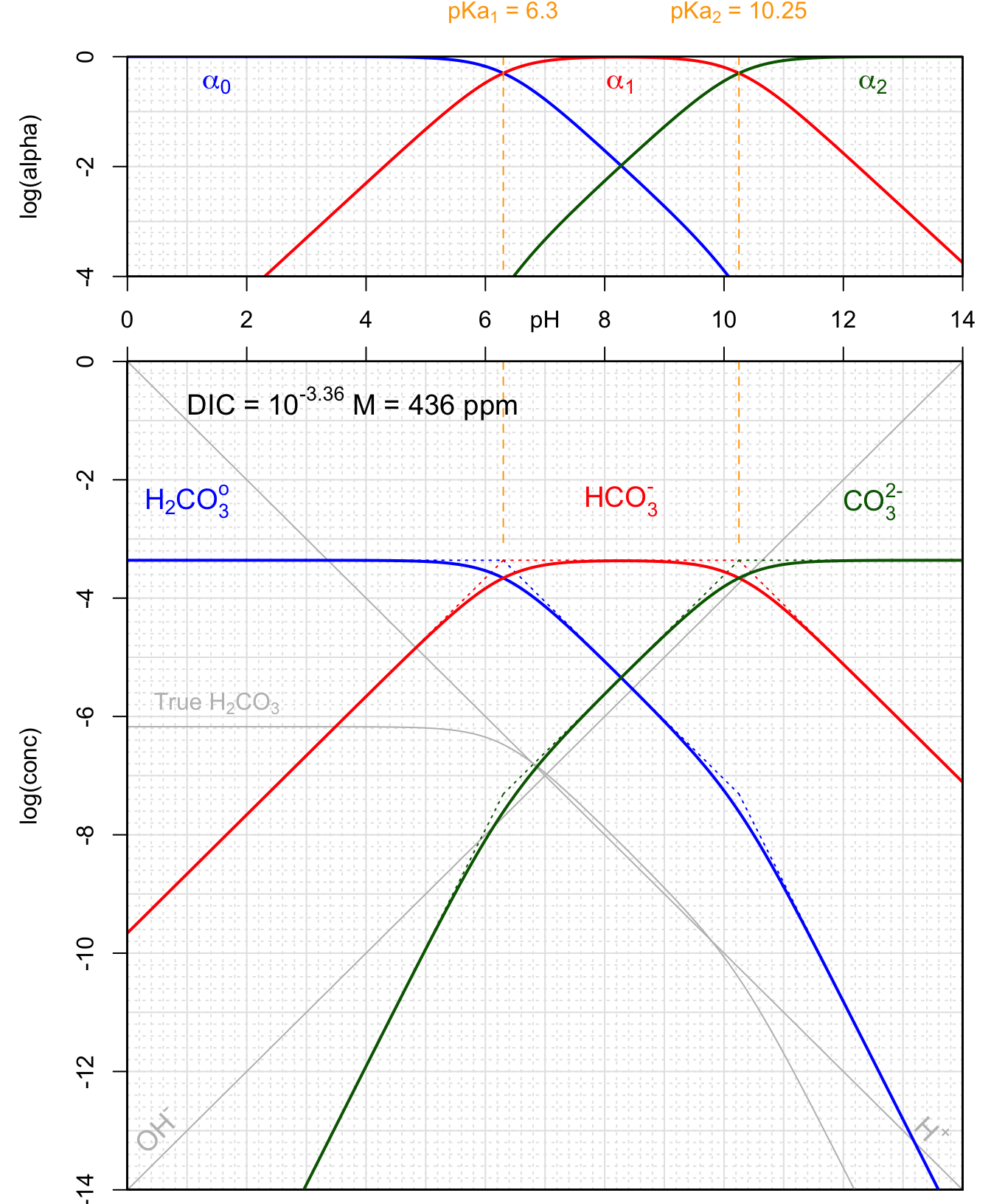
Figure 11.18: Carbonates and conjugate acids in a closed system for total concentration of 10^-3.4M as a function of pH at 25°C

Bjerrum plot

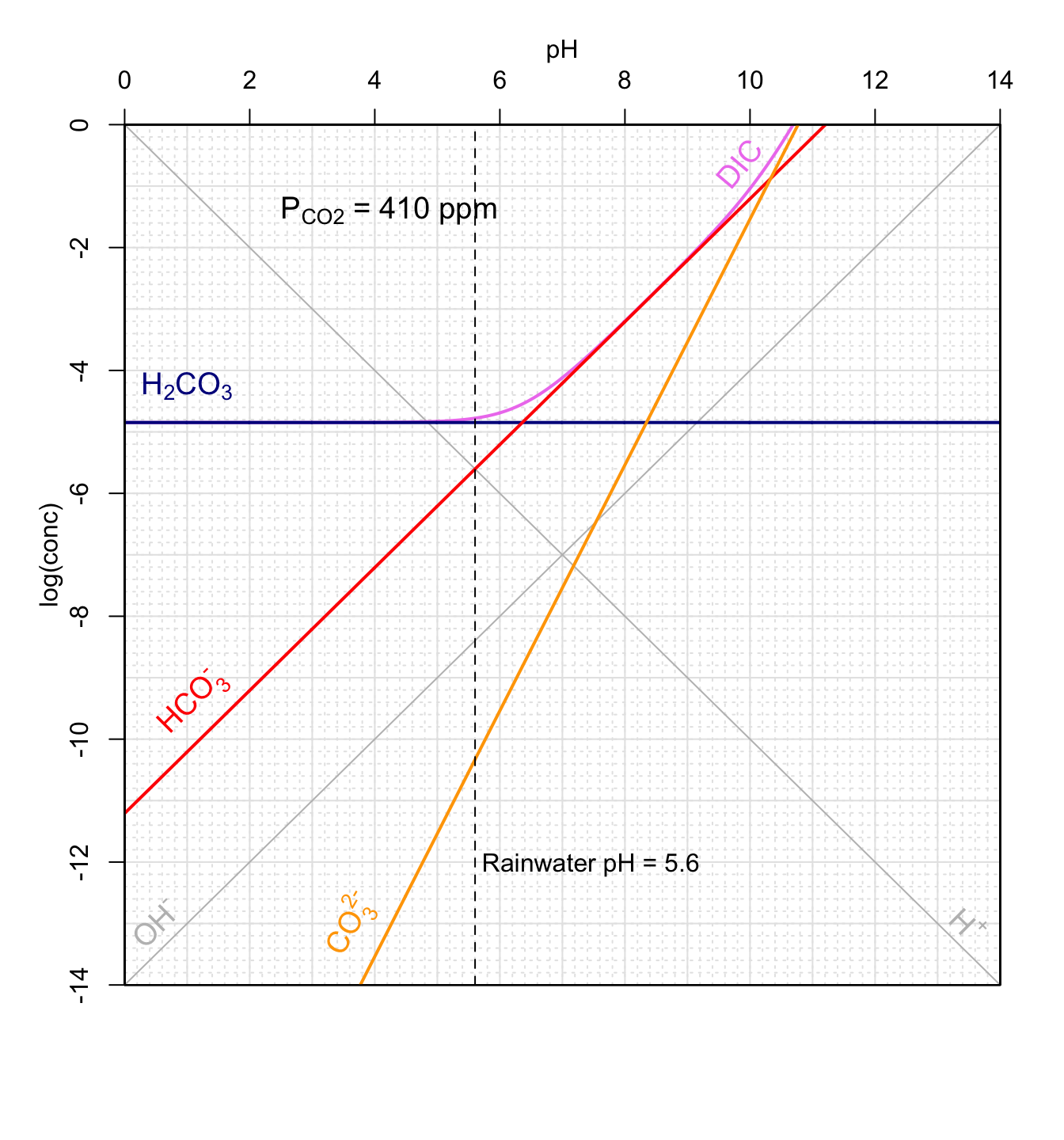
Figure 11.19: Concentrations of carbonates and conjugate acids in an open system in equilibrium with atmospheric CO₂ as a function of pH at 25°C. Graphical method to calculate theoretical pH of rainwater

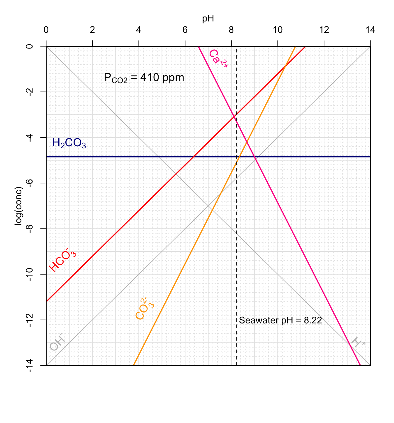
Figure 11.20: Concentrations of carbonates and conjugate acids in an open system in equilibrium with atmospheric CO₂ as a function of pH at 25°C. Graphical method to calculate theoretical pH of rainwater

Figure 11.21: Decrease of seawater pH as a function of increasing \(P_{CO_2}\) in the atmosphere using the graphical method introduced above

This chapter is still under construction

References

Barker, J C, J P Zublena, and F R Walls. 1994. “Animal and Poultry Manure Production and Characterization.” North Carolina Cooperative Extension Service.

Harned, Herbert S, and Benton B Owen. 1958. The Physical Chemistry of Electrolytic Solutions. Reinhold Pub. Corp.

Henry, William, and Joseph Banks. 1803. “III. Experiments on the Quantity of Gases Absorbed by Water, at Different Temperatures, and Under Different Pressures.” Philosophical Transactions of the Royal Society of London 93 (January): 29–274. https://doi.org/10.1098/rstl.1803.0004.

Stumm, Werner, and James J Morgan. 1996. Aquatic Chemistry: Chemical Equilibria and Rates in Natural Waters. Wiley. https://market.android.com/details?id=book-xvZOAAAAMAAJ.