Chapter 13 Dissolved gases in water

Chapter summary:

Let us admit it: dissolved gases have been a bit of a mystery for all of us at one point. There have been many articles written and a book has recently been published (Colt 2012) on the subject giving all the numbers and constants one could dream of…! So the subject is both relatively simple in principle but far from simple in the details. This chapter presents the principles and enough, and hopefully not too much, of the details.

When one sees sparkling water, it is obvious that there is gas dissolved in it as bubbles form on their own and one can see them form and escape. They also apparently seem to form more when the water temperature is warm than when a sparkling water bottle just comes out of the fridge (Figure 13.1).

Figure 13.1: Dissolved gas bubble formation from a sparkling water bottle at 4°C and 25°C

Figure 13.1 shows that temperature has to do something with how gases may dissolve in water. At warm temperature, the opening of the sparkling water bottle is accompanied by the release of gas under pressure in the bottle headspace and the sudden formation of many bubbles. At low temperature, the gas release upon opening is not nearly as high, and the number of bubbles forming and bubbling up is much lower.

Another observation is that before the opening of the bottle, there are few bubbles apparent on the bottle sides, so under some pressure in the headspace, the gases appear to stay dissolved, and it is only after the bottle has been opened and that the bottle headspace is at atmospheric pressure that gas bubbles appear ‘from no where’ in a process called ebullition. This simple experience thus shows several things:

• at low and high temperatures, the pressure in the bottle headspace is respectively lower and higher, suggesting that there is more gas in the head space at higher temperature, and thus more dissolved gases at lower temperatures
• as the headspace pressure is released, gases are released suggesting that more gas can be dissolved in water when water is under pressure. We shall see what this really means later in this chapter

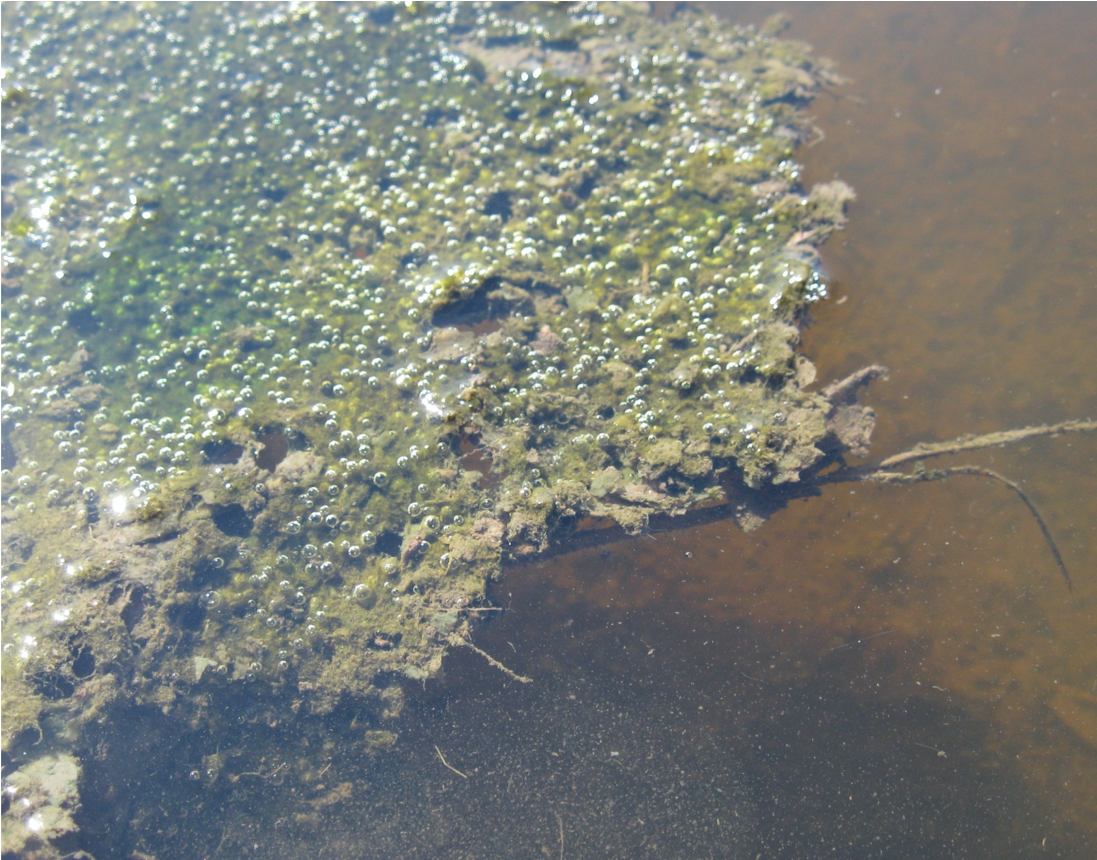
Figure 13.2: Formation of gas bubbles attached to a biofilm (periphyton) scraped from an organic sediment in a tidal marsh

There are other interesting observations to consider. You might have already observed bubble formation in a stream during Spring or Summer a bit like in the picture in Figure 13.2. These bubbles are attached to a biofilm scraped from a stream bottom in North Carolina. Obviously, the presence of bubbles is not necessarily very informative about dissolved gases, but the sparkling water experience above suggests that in reality, if there are bubbles, there must necessarily be dissolved gases associated.

Figure 13.3: Gas bubbling from the sediment of a low gradient stream when disturbed

One last introductory experience you might have had, is the release of gas bubbles when you might have disturbed the sediment of a wetland or a stream sediment when you stepped on it a bit like in the above video (Figure 13.3). Obviously, gases must have accumulated in the sediment and it took some disturbance to release them. This suggests that there are gas formation processes in treatment systems, but that we already knew (see Chapter on sediment redox processes). The additional information is how gases dissolve or form bubbles.

So this chapter explores the conditions for which gases dissolve or form bubbles, the driving factors behind, and the consequences for biogeochemical processes.

13.1 Henry’s law and the dissolution of gases in water

English chemist William Henry published his results from his experiments on the dissolution of gases in 1803 (Henry and Banks 1803), and reported in page 42 of the January 1803 issue of the Philosophical Transactions of the Royal Society of London that

[…] it follows, that water takes up, of gas condensed by one, two, or more additional atmospheres, a quantity which, ordinarily compressed, would be equal to twice, thrice, &c. the volume absorbed under the common pressure of the atmosphere (Henry and Banks 1803).

In other words, Henry’s law states that the amount of dissolved gas in a liquid is proportional to its partial pressure above the liquid. The winner of first Nobel price in Chemistry (1901), Dutch chemist Jacobus Henricus van’t Hoff later formulated in 1884 how the dissolution of the gases depends on the temperature, in what is now referred to as the van’t Hoff equation (equation (13.2); van’t Hoff (1884)). Henry’s law has several important consequences for ecological engineering:

1. knowing the partial pressure of a gas in the atmosphere, it is possible to calculate the concentration of that gas in water, at least at equilibrium.
2. it is possible to then compare the concentrations of gases in one liter of atmosphere versus those of one liter of water
3. it is possible to calculate, for any given dissolved gas, what the equivalent partial pressure would be if it were at equilibrium with the atmosphere, and realize the reasons for the formation of bubbles in treatment systems (referred to as ebullution)
4. realize that gases can be in ‘supersaturation’ in water, i.e., have more dissolved gases than when in equilibrium with the atmosphere, because of hydrostatic pressure, and/or because of the kinetics of gas production in treatment systems vs. the kinetics of equilibrium of gases with the atmosphere

13.1.1 Equivalence between gas partial pressures and dissolved concentration

Henry’s law stipulates that the concentration in the aqueous phase \(c_a\) (subscript \(a\) for aqueous) of a dissolved gas A, i.e., the number of gas moles per liter of water, can be calculated as:

\[\begin{equation} c_a(A) = K^{cp}_H(A).p_A \tag{13.1} \end{equation}\]

where \(c_a(A)\) is the concentration of dissolved gas A in water (\(c\) stands for concentration and the subscript \(a\) stands for aqueous), \(K^{cp}_H(A)\) is the Henry’s constant for gas A and at a given temperature, and \(p_A\) is the partial pressure of gas A in the head space above water. The use of \(K^{cp}_H\) here does not follow notation that might be found elsewhere (e.g., in Sander (2015) or on Wikipedia, where \(K^{cp}_H\) would be written as \(H^{cp}\)). This notation has been chosen here to correspond to the notation traditionally used in thermochemistry where equilibrium constants are noted “K”, and the subscript “H” refers to Henry (e.g., Stumm and Morgan (1996)), and also because the letter \(H\) also refers to as enthalpy in thermodynamics… The superscript \(cp\) in \(K^{cp}_H\) means that this Henry’s law constant yields an aqueous concentration (\(c\)) when multiplied by a gaseous pressure (\(p\)). Equation (13.1) thus characterize how soluble a gas is as a function of its pressure above in the gaseous phase. As a result, \(K^{cp}_H\) is referred to as a Henry’s law solubility constant.

13.1.2 Many different units to express gas solubility

This is where things can start to be a bit confusing, as there are many ways of expressing the way gases behave with aqueous systems. One may be interested on how gases may dissolve in the aqueous phases (the term solubility is then used), or instead how gases may escape the aqueous system (the term volatility is then used) (e.g., Markham and Kobe 1941; Colt 2012; Sander 2015). In both cases, Henry’s law apply but the solubility and volatility constants are inverse of each other. As far as we are concerned, we will use Henry’s law solubility constants and ignore the volatility constants. In Equation (13.1) dissolved concentrations would be expressed in mol.L^-1 (liter of water), pressures expressed in atm, which leaves the Henry’s solubility constant units to be mol.L^-1.atm^-1. That is the simple approach and this is in many cases enough.

To be a bit more rigorous, however, one should speak about dimensions and then give potential units. So, Equation (13.1) expresses the dissolved gas concentration, which dimensions are [Mass.Volume^-1] or more properly [M.L^-3], where M is the letter for Mass, and L for length. In our domain of science, common units for concentrations are mol.L^-1 or mg.L^-1. The dimension of the partial pressure is [M.L^-1.T^-2], which is the equivalent of a force [M.L.T^-2] spread over a surface [L^-2], and where “T” refers to ‘Time’. Common units for pressures are atmosphere (atm), bars (bar), although the SI unit is called the Pascal (Pa), and the correspondence being 1 atm = 1.01325 bar = 101,325 Pa. As a result the dimensions for the Henry’s law solubility constant in Equation (13.1) are [M².L^-1.T^-2], or more simply in common units mol.L^-1.atm^-1 as already mentioned. This or similar unit is the one that is more relevant to the domain of ecological engineering and the values for relevant gases are consigned in the first two columns of Table 13.1 below.

Table 13.1: Henry’s law Constants of Importance in Gas-Water Equilibria at 25°C (values from Sander (2015) and www.henrys-law.org). \(k^{cp}_H\) and \(K^{cp}_H\) correspond to Henry’s solubility constants expressed in slighlty different units, \(K^{cc}_H\) is the unitless Henry’s solubility constant, calculated as the ratio \(c_a/c_g\), and \(TempConst\) corresponds to the van’t Hoff equation temperature factor described in the text

Reactions	\(\frac{k^{cp}_H(25°C)}{(mol.m^{-3}.Pa^{-1})}\)	\(\frac{K^{cp}_H(25°C)}{(M.atm^{-1})}\)	\(\frac{Temp Const}{(°K)}\)	\(\frac{K^{cc}_H}{(unitless)}\)
\(He_{(g)} \rightleftharpoons He_{(aq)}\)	3.80e-06	3.85e-04	230	0.9%
\(Ne_{(g)} \rightleftharpoons Ne_{(aq)}\)	4.40e-06	4.51e-04	490	1.1%
\(Ar_{(g)} \rightleftharpoons Ar_{(aq)}\)	1.40e-05	1.42e-03	1300	3.5%
\(H_{2(g)} \rightleftharpoons H_{2(aq)}\)	7.80e-06	7.85e-04	500	1.9%
\(O_{2(g)} \rightleftharpoons O_{2(aq)}\)	1.25e-05	1.27e-03	1700	3.1%
\(CO_{(g)} \rightleftharpoons CO_{(aq)}\)	9.70e-06	9.83e-04	1300	2.4%
\(CO_{2(g)} \rightleftharpoons CO_{2(aq)}\)	3.35e-04	3.39e-02	2400	83%
\(CH_{4(g)} \rightleftharpoons CH_{4(aq)}\)	1.40e-05	1.42e-03	1600	3.5%
\(H_{2}S_{(g)} \rightleftharpoons H_{2}S_{(aq)}\)	1.00e-03	1.01e-01	2100	247.9%
\(N_{2(g)} \rightleftharpoons N_{2(aq)}\)	6.40e-06	6.48e-04	1300	1.6%
\(N_2O{(g)} \rightleftharpoons N_2O{(aq)}\)	2.40e-04	2.43e-02	2600	59.5%
\(NH_{3(g)} \rightleftharpoons NH_{3(aq)}\)	5.90e-01	5.98e+01	4200	146250.3%

Yet, glancing through the values of the first and second columns of Table 13.1 might not necessarily trigger a big eureka, I understand how gas dissolve in water now…! Possibly a more telling approach is the comparison between the concentrations in the gaseous versus those in the aqueous phases. This is what the dimensionless Henry’s solubility constant \(K^{cc}_H\) does. This constant expresses the ratio between the concentrations (number of moles per liter) in the aqueous phase (\(c_a\)) over those in the gaseous phase (\(c_g\)), such that in the end \(K^{cc}_H = \frac{c_a}{c_g}\) (the superscript \(cc\) in \(K^{cc}_H\) stands for concentration to concentration). This constant is dimensionless and can be expressed as a percentage value as reported in Table 13.1.

Before discussing the values, visualizing the \(c_a\) and \(c_g\) concentrations aqueous and gaseous phases might help. Let us imagine containers that would be 2 liters in volume each, and containing 1 liter of water and 1 liter of gas head space above (Figure 13.4). The gaseous phase of the containers would be at 1 atm and filled with one pure gas only. Now to visualize the ratio of the number of moles in both phases, Henry’s law solubility constants in the first and second columns of Table 13.1 give the number of moles of gas dissolved per liter of water, assuming that the overlying gas is pure and at one atmosphere. The concentration in the gaseous phase can be calculated using the perfect gas law, which yields that at 25°C, one mole of gas takes about 24.47 liters, so the concentration in one liter of gas is \(1/24.47 = 40.87 mmol.L^{-1}\). More calculation details are provided in Exercise 13.1 below.

The \(\frac{c_a}{c_g}\) or \(\frac{liquid}{gas}\) ratio for \(O_2\), \(N_2O\), and \(CO_2\) gases is illustrated in Figure 13.4A, B, and C, respectively, with 100 random points in the gaseous phase representing the 40.9 mmol.L^-1 of gases present in 1L at 1atm, and, the corresponding 3, 59, and 83 points representing the respective gaseous concentrations \(c_g\). The ratios displayed at the bottom of the figure apply for water temperature at 25°C.

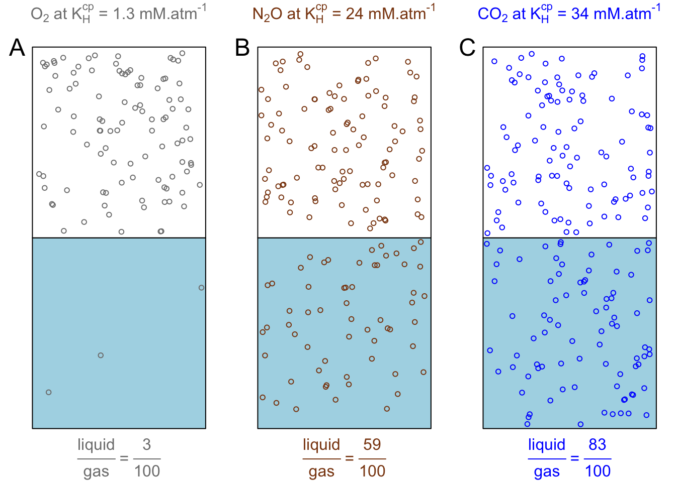
Figure 13.4: Visual and liquid:gas proportions of the number of moles in the gaseous phase of one liter of gas at 1 atm overlying one liter of water, for O₂, N₂O, and CO₂ gases, using the respective Henry’s solubility constants at 25°C. Blue rectangles represent one liter of water in equilibrium with one liter of pure gas (overlying white rectangle). There are 100 circles in the white rectangle representing the 40.9 mmol.L^-1 of gases present in 1L at 1 atm at 25°C. The number of circles in the blue rectangles represent the respective and corresponding number of moles per liter of water

Actually, the dimensionless Henry’s solubility constants reported at 25°C in the fourth column of Table 13.1 are valid regardless of the pressure in the gaseous phase. The numbers reveal two strikingly different types of gases: insoluble and soluble gases. All perfect gases reported as well as linear or non-polar molecules such as \(O_2\), \(N_2\), or \(CH_4\) are generally referred to as insoluble as at 25°C, and which concentrations in water are less than 3.5% those in the atmosphere above. Reversely, polar molecules such as \(H_2S\), \(N_2O\) and \(NH_3\) are very to extremely soluble. Ammonia and hydrogen sulfide are very polar molecules, with the S and N strongly electronegative and the hydrogen atoms electropositive, hence the ability to make very strong hydrogen bonds and the very high solubility of these two gases. \(N_2O\) also is polar as two Lewis dot structures coexist (\(N\equiv \overset{+}{N}-O^- \longleftrightarrow {}^-N=\overset{+}{N}=O\)), and in both cases, the center nitrogen atom is positevely charged and either the other nitrogen or the oxygen atoms are negatively charged.

Carbon monoxide and dioxide are oddities. The carbon monoxide molecule is asymmetrical with a triple bond between the two atoms and one lone pair of electrons on each atom (:C≡O:). It turns out that despite the more electronegative oxygen atom, it is the carbon atom that is slightly more negative than the oxygen (Sato et al. 2000). As a result, hydrogen bonds do not form readily, but a little more than for \(N_2\), and less than for \(O_2\). The linear O=C=O carbon dioxide molecule does not have a net dipole but the carbon has an effective positive charge. It appears that experiments have shown that there are specific hydrogen bonding between the water molecule and the \(CO_2\) molecules (Sato et al. 2000), which renders carbon dioxide to be very soluble. The nature of these specific hydrogen bonding is not clear. The hydration of \(CO_2\) to carbonic acid (see details in Chapter 11) does not occur very much and cannot be a major factor to explain \(CO_2\) high solubility.

There are additional units to express Henry’s solubility constants, which appear to depend on the scientific domains and applications. For example, a more universal dimension, which oceanographers preferably use is the solubility constant [Mass_of_dissolved_gas.Mass_of_water^-1] often expressed as mol.kg^-1 (kg of water). In freshwater systems one liter of water weighs very close to 1 kg, but for sea or brackish waters, the weight of water varies with salinity and it is more robust to express solubility in [Mass_of_dissolved_gas.Mass_of_water^-1].

Another dimension/unit used for gases under pressure in water is [Volume_of_dissolved_gas.Volume_of_water^-1] often expressed in mL.L^-1 or L.L^-1 (essentially dimensionless as well). This unit can be quite confusing. So this corresponds to the volume of gas (at one atm) that would be extracted (if one could) per unit volume of water. The Bunsen coefficient \(\alpha\) is an application of this unit when temperature is at 0°C or 273.15°K and pressure at 1 atm. Examples presented in Exercise 13.1 clarify the correspondence between all the units presented here. A full list of all units used for Henry’s constants and the correspondence between them all is available in Colt (2012) and Sander (2015).

Exercise 13.1

Calculate solubility in freshwater of pure O₂, N₂, and CO₂ at 1 atm and 25°C in different units

Let us take one liter of pure freshwater overlaid by one liter of pure gas at 1 atm. To calculate the solubility of these gases, one needs to just use the Henry’s law in the equation

\[\begin{equation} c_a = K^{cp}_H.p \end{equation}\]

In this exercise the gas partial pressure is equal to 1 atm. The unit available and given in Table 13.1 for \(K^{cp}_H\) is M.atm^-1, i.e., mol.L^-1.atm^-1. Using Henry’s law and solubility constants, one can calculate the solubility values expressed in different units at 25°C:

• \(K^{cp}_H(O_2)=1.27 \space 10^{-3} mol.L^{-1}.atm^{-1}\)
• \(K^{cp}_H(N_2)=6.48 \space 10^{-4} mol.L^{-1}.atm^{-1}\)
• \(K^{cp}_H(CO_2)=3.39 \space 10^{-2} mol.L^{-1}.atm^{-1}\)

Solubility in \(mol.L^{-1}\)

• \([O_{2(aq)}] = 1.27 \space 10^{-3} \times 1 = 1.27 \space 10^{-3} \space mol.L^{-1}\)
• \([N_{2(aq)}] = 6.48 \space 10^{-4} \times 1 = 6.48 \space 10^{-4} \space mol.L^{-1}\)
• \([CO_{2(aq)}] = 3.39 \space 10^{-2} \times 1 = 3.39 \space 10^{-2} \space mol.L^{-1}\)

the \(\times 1\) in the above equations correspond to pressure at 1 atm.

Solubility in \(mol.kg^{-1}\)

To express solubilities in mol.kg^{-1}, one must multiply the above results by the density of water at 25°C. The density, in \(kg.m^{-3}\), of water as a function of temperature for the range 5°C to 40°C can be expressed as (Jones and Harris 1992):

• for air-free water: \(\rho = 999.85308 + 6.32693 \times 10^{-2}.t - 8.523829 \times 10^{-3}.t^2 + 6.943248 \times 10^{-5}.t^3 \\ -3.821216\times 10^{-7}.t^4\)
• for air-saturated water: \(\rho = 999.84847 + 6.337563 \times 10^{-2}.t - 8.523829 \times 10^{-3}.t^2 + 6.943248 \times 10^{-5}.t^3 \\ -3.821216\times 10^{-7}.t^4\)

Using the air-saturated equation, the density of freshwater at 25°C would be \(\rho = 0.997041 \space kg.L^{-1}\)

• \([O_{2(aq)}] = 1.27 \space 10^{-3} \div 0.997041 = 1.27 \space 10^{-3} \space mol.kg^{-1}\)
• \([N_{2(aq)}] = 6.48 \space 10^{-4} \div 0.997041 = 6.50 \space 10^{-4} \space mol.kg^{-1}\)
• \([CO_{2(aq)}] = 3.39 \space 10^{-2} \div 0.997041 = 3.40 \space 10^{-2} \space mol.kg^{-1}\)

Unitless Henry’s solubility constant

To calculate the ratio of aqueous vs. gaseous concentrations, one needs to first calculate the concentration of each gas in the head space at 1 atm. For that, we use the ideal gas equation:

\[\begin{equation} PV = nRT \\ V = \frac{nRT}{P} \end {equation}\]

Using the conditions where

• \(P = 1 \: atm = 101,325 Pa\),
• \(n = 1 \: mol\),
• \(R = 8.314 \space m^3⋅Pa⋅K^{−1}⋅mol^{−1}\), and
• \(T = 25°C = 298.15°K\)

\[\begin{equation} V = \frac{1 \times 8.314 \times 298.15}{101,325} \end {equation}\]

Assuming perfect gases, one mole of gas would occupy 24.46 L. In other words, in one liter of gas at 1 atm, there are \(1/24.46 = 4.09.10^{-2}\) moles of gas.

From this, it is possible to calculate the unitless Henry’s solubility constant \(K^{cc}_H\) by dividing the aqueous concentrations by the gaseous concentration ( \(\frac{c_a}{c_g}\)). This yields:

• \(K^{cc}_H(O_2) = \frac{1.27.10^{-3}}{4.09.10^{-2}} = 3.1\%\)
• \(K^{cc}_H(N_2) = \frac{6.48.10^{-4}}{4.09.10^{-2}} = 1.6\%\)
• \(K^{cc}_H(CO_2) = \frac{3.39.10^{-2}}{4.09.10^{-2}} = 82.9\%\)

Solubility in \(ml.L^{-1}\)

This unit expresses the volume of gas that could be extracted from a solution, and that volume at 1 atm. To calculate solubility in this unit, one just needs to multiply the \(K^{cp}_H\) solubility constant by the molar volume of a real or perfect gas. Assuming to deal with a perfect gas,

• \(Vol_{O_{2(aq)}} = 1.27.10^{-3} \times 24.46 = 31.1 mL.L^{-1}\)
• \(Vol_{N_{2(aq)}} = 6.48.10^{-4} \times 24.46 = 15.9 mL.L^{-1}\)
• \(Vol_{CO_{2(aq)}} = 3.39.10^{-2} \times 24.46 = 829 mL.L^{-1}\)

These values also correspond to \(10 \times K^{cc}_H\). in reality, actual gases do not behave like perfect gases and actual molar volumes differ a little bit. Approximating actual gases to perfect gases is good enough for our purpose.

In reality the concept of solubility extends beyond gases in liquid, and “is the property of a solid, liquid or gaseous chemical substance called solute to dissolve in a solid, liquid or gaseous solvent” (Wikipedia contributors 2020c). In most cases the solvent is a liquid. As the activity of solute and solvents vary with temperature, the solubility of gases in water varies with temperature, and the van’t Hoff equation is the formulation of this relationship.

13.2 Solubility of gases as a function of temperature {#sol-f-temp)}

Everyone has experienced the consequences of opening a can of soda coming from the fridge or coming from a car having spent some time under a hot sun in summer, and a less dramatic effect is illustrated in Figure 13.1… As a recall, in the first case, opening the can makes a small noise as this releases a little bit of gas (largely corresponding to the extra \(CO_2\) forcefully dissolved under 4 bars at 4°C during bottling). In the second case, it will be a very noisy mess as bubbles of soda will try to violently escape! This experience shows that the pressure of gas in the headspace in the cans is much higher under warm than under cold temperatures. Because all the cans are bottled under the same cold conditions hence containing about the same number of moles of gases, the number of moles of dissolved gas under cold conditions is greater than under warm ones.

Henry’s law as formulated in equation (13.1) applies for any given temperature. Henry’s constant is the parameter that changes with temperature. The van’t Hoff equation gives the values of Henry’s constant for any given temperature (equation (13.2)):

\[\begin{equation} K^{cp}_H(T) = K^{cp}_H(T_0).exp \left[ \left( \frac {-\Delta_{sol}H}{R} \right) \left( \frac{1}{T} - \frac{1}{T_0} \right) \right] \tag{13.2} \end{equation}\]

where \(K^{cp}_H(T)\) and \(K^{cp}_H(T_0)\) represent the Henry’s solubility constants, respectively for \(T\) and the \(T_0\) (in °K), the latter being the reference temperature (usually at 25°C or 298.15°K), \(\Delta_{sol}H\) represents the enthalpy of dissolution, \(R\) is the perfect gas constant (8.314 J.mol⁻¹.K⁻¹)². The values for the term \(\frac {-\Delta_{sol}H}{R}\) in equation (13.2) represent a temperature constant in Kelvin and depend on the gases. In the form above, the van’t Hoff equation is only valid for a limited temperature range in which \(\Delta_{sol}H\) does not change much with temperature, which is the case for natural waters (Sander 2015).

Again, the term \(\frac {-\Delta_{sol}H}{R}\) represents a temperature constant, which values are summarized in Table 13.1 under the column heading TempConst. The values of the Henry’s law constant at reference temperature \(K^{cp}_H(T_0)\) are summarized using the SI (SI, abbreviated from the French Système international (d’unités)) units (\(mol.m^{-3}.Pa^{-1}\)) and practical units (\(M.atm^{-1}\), i.e., \(mol.L^{-1}.atm^{-1}\)) in Table 13.1. All values have been obtained from Sander (2015), which are regularly updated on www.henrys-law.org.

Using the van’t Hoff equation to predict Henry’s constants for any given temperature, it is possible to plot the solubility (in mol.L^-1 in water) of common gases relevant to ecological engineering between 0 and 40°C (Figure 13.5A). These solubility values are calculated for pure gases at 1 atm of pressure and are thus comparable from one to another (the actual solubilities for normal air at 1 atm are illustrated in Figure 13.6). Notice that the solubility values for \(CO_2\), \(H_2S\) and \(N_2O\) are plotted in dotted lines and are read on the secondary Y-axis. Solubility values for these gases are 10 to 50 times larger than the ones for \(O_2\), \(H_2\), \(N_2\), \(CO\), and \(CH_4\), which are plotted as solid lines.

Exercise 13.2

Formula of the solubility of pure O₂ at 1 atm as a function of temperature T in °C

To express this formula, one needs to combine Henry’s law and van’t Hoff equations:

\[\begin{equation} [O_{2(aq)}] = K_H(T_0).exp \left[ \left( \frac {-\Delta_{sol}H}{R} \right) \left( \frac{1}{T} - \frac{1}{T_0} \right) \right].P_{O_2} \end{equation}\]

The values for the terms \(K_H(T_0)\) (in mol.L^-1.atm^-1) and \(\frac {-\Delta_{sol}H}{R}\) (in °K) are provided in Table 13.1. The van’t Hoff equation uses temperature in °K. The conversion equation is \(T(°K) = T(°C) + 273.15\). A partial numerical application of this equation for dissolved oxygen expressed in mol.L^-1 in one liter of water overlaid by one liter of pure oxygen at 1 atm using T in °C would yield:

\[\begin{equation} [O_{2(aq)}] = 1.27 \space 10^{-3}exp \left[ 1700\left( \frac{1}{T+273.15} - \frac{1}{25+273.15} \right) \right] \times 1 \end{equation}\]

In Figure 13.5B, the ratio of the number of moles in water and those in the overlying gas are calculated by dividing the solubility in mol.L^-1 displayed in Figure 13.5B, by the number of moles in the overlying gaseous phase. This number varies with temperature, and is calculated using the ideal gas equation as \(n = \frac{PV}{RT}\) where all letters and values are defined in Exercise 13.1.

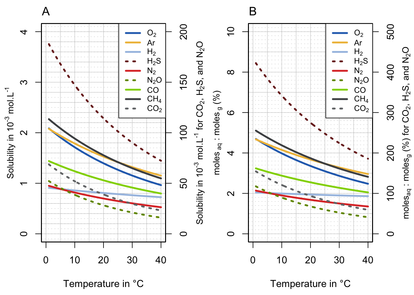
Figure 13.5: Solubility plots for common gases relevant to ecological engineering expressed in mol.L^-1 (A) and unitless % as the ratio of \(c_a/c_g\) (B). Each gas is assumed to be at 1 atm of pressure in the gaseous phase. Notice that the value for \(CO_2\), \(H_2S\) and \(N_2O\) are read on the secondary Y-axis

These plots show several striking results. First, they confirm that \(O_2\), \(H_2\), \(N_2\), \(CO\), and \(CH_4\) do not dissolve well into water, regardless of temperature, as no more than 2% to 5% of the molecules in the gaseous phase are dissolved at equilibrium. For dioxygen gas, at 10°C and 25°C, respectively 4% and 3% of \(O_2\) present in the atmosphere above are dissolved in water. This suggests that the mere amount of dioxygen in an aquatic milieu is rather limited and about 30 times less than what is available in a gaseous milieu. Although life seems to have sprung in water, it is clear that it was a lot more advantageous for organisms to live in a gaseous milieu for this reason. But then organisms had to find ways to obtain water, and not lose it, hence the plethora of adaptations from organisms to adapt to these relatively dry conditions.

For ecological engineering purposes, this observation is one of the main reasons why \(O_{2(aq)}\) is limited in water and why the respiratory demand for oxygen in treatment systems tends not to be matched by supply, hence the very common presence of anaerobic zones (more details in section 8.2).

Second, contrary to the previous gases, \(CO_2\), \(H_2S\), and \(N_2O\) readily dissolve in water to the point that at 10°C, there are more moles of \(CO_2\) and \(H_2S\) dissolved in water than there are in the overlying atmosphere, respectively about 1.2 and 3.5 times more! At the same temperature, there is almost the same number of moles of \(N_2O\) dissolved in water (90%) as there are in the gaseous phase. This also means that at 10°C one could extract 1.2 L of CO₂ out of 1 L of water!

Exercise 13.3

Calculate the volume of CO₂ stored in a bottle of Champagne at 10°C

First, one needs to know that the volume (\(V_{ch}\)) of liquid in a bottle of Champagne is 75 cL or 0.75 L. Second, people have actually measured the pressure in the headspace pressure (\(p_{CO_2}\)) and it easily reaches 5 bars (≈72 psi). Pressure in a car tire is about 2.2 (≈32 psi) bars, for comparison. This is why the corks on a bottle of Champagne are maintained with a wire to prevent corks to pop out on their own! But why is there pressure in there? Most of the gas under pressure is actually CO₂ resulting from the fermentation processes.

To calculate the actual solubility is far from easy because the wine composition itself has an impact on solubility… One of the sought after quality of a Champagne wine is the size of the gas bubbles that form: the smaller the better, and that is a fine art. This is not the goal of this exercise. We shall approximate the Champagne wine to be pure water and that all the dissolved gas is CO₂. In reality, we know that there is no oxygen because of the fermentation. There is dinitrogen most likely at equilibrium with the atmosphere when the grapes were pressed. But we will take this to be negligible.

From the information given above, the dissolved CO₂ concentration can be calculated as:

\[\begin{equation} [CO_{2(aq)}] = K^{cp}_H(T_0).exp \left[ \left( \frac {-\Delta_{sol}H}{R} \right) \left( \frac{1}{T} - \frac{1}{T_0} \right) \right] \times p_{CO_2} \end{equation}\]

using the terms defined previously. The number of dissolved moles in the bottle is thus \(n_{CO_{2(aq)}} = [CO_{2(aq)}] \times V_{ch}\). The volume taken by this number of moles is thus \(V_{CO_2} = n_{CO_{2(aq)}} \times Vol_{PerfectGas}(T)\)

Overall, the volume of CO₂ stored in a bottle of Champagne at 10°C could be calculated as:

\[\begin{equation} V_{CO_2} = K^{cp}_H(T_0).exp \left[ \left( \frac {-\Delta_{sol}H}{R} \right) \left( \frac{1}{T} - \frac{1}{T_0} \right) \right] \times p_{CO_2} \times V_{ch} \times \frac{RT}{P} \end{equation}\]

Using:

• \(T_0\) = 25°C = 298.15°K, \(K^{cp}_H(T_0) = 3.39 \space 10^{-2} mol.L^{-1}.atm^{-1}\)
• \(T\) = 10°C = 283.15°K
• \(\frac {-\Delta_{sol}H}{R} = 2400°K\)
• \(p_{CO_2}\) = 5 bars = 5/1.01325 atm
• \(V_{ch}\) = 0.75 L
• \(P = 1 \: atm = 101325 Pa\),
• \(R = 8314 \space L⋅Pa⋅K^{−1}⋅mol^{−1}\)

\[\begin{equation} V_{CO_2} = 3.39 \space 10^{-2}.exp \left[ 2400 \left( \frac{1}{283.15} - \frac{1}{298.15} \right) \right] \times \frac{5}{1.0325} \times 0.75 \times \frac{8314 \times 283.15}{101325} \end{equation}\]

\(V_{CO_2} = 4.47 L\)

The temperature chosen to calculate the molar volume of a perfect gas was chosen to be 10°C like the water temperature. Another value could have been chosen to possibly represent room temperature. Yet, it is remarkable to realize how much CO₂ can be dissolved in sparkling water, and in the case of spakling wine or beer, that most of the CO₂ was produced by microbes through fermentation

13.3 Actual solubility values of water in equilibrium with the atmosphere

Now, it is time to look at the actual solubilities and concentrations of four of the most abundant gases in the atmosphere (excluding water vapor, considered to be at 1% at sea level and 0.4% overall in the atmospher): dinitrogen (78%), dioxygen (21%), argon (9,340 ppm or 0.934%), and carbon dioxide (415 ppm in 2020). Dinitrogen is among the least soluble gases (Figure 13.5), but because it comprises the vast majority of the atmosphere (78%), its overall actual solubility expressed in mmol.L^-1 is the highest and about 1.5 times that of dioxygen (Figure 13.6). The second most dissolved gas is O₂, the third is CO₂, and the fourth is argon (Figure 13.6).

Solubility of argon at 1 atm is about 1.14 times that of oxygen, but its actual solubility is lower than CO₂, despite the fact that its partial pressure in the atmosphere is about 23 times that of CO₂ in 2020. Solubility of CO₂ at 1 atm is about 30 times higher than that of O₂, but in year 2020 the atmospheric concentration was about 415 ppm or 0.0415% or about 500 times less than the 21% of O₂. In the end, the theoretical solubility of CO₂ in water is about 17 times lower than that of O₂, which is remarkable for a gas that is 500 times less present in the atmosphere! Do not forget, however, that some of the CO₂ becomes hydrated into carbonic acid and dissociates into carbonates. But as we saw in the chapter dedicated to dissolved carbon dioxide, the dissociation into carbonates does not influence, in an open system, the concentration of dissolved CO₂.

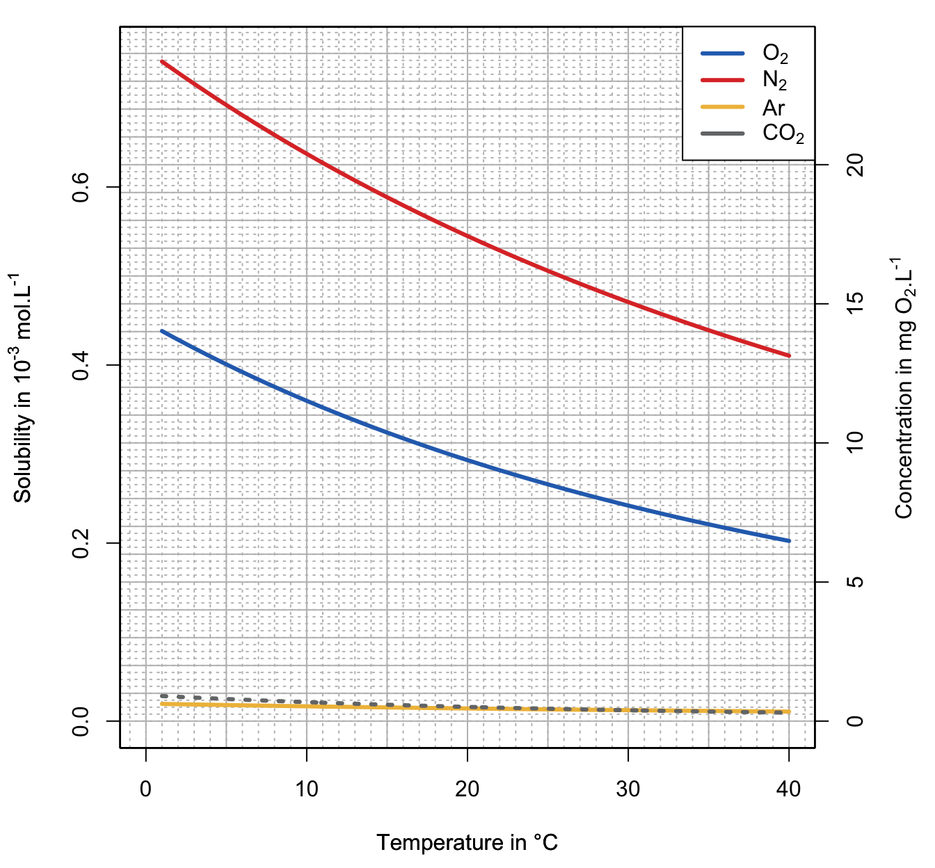
Figure 13.6: Solubility graph for \(N_2\), \(O_2\), and \(CO_2\) at equilibrium with the atmosphere, assuming \(P_{N_2} = 0.78 atm\), \(P_{O_2} = 0.21 atm\), and \(P_{CO_2} = 410 ppm\). Dissolved \(O_2\) concentration, i.e., where the partial pressure of \(O_2\) is equal to 0.21 atm. The corresponding concentrations in mg O₂.L^-1 are read on the secondary axis

Obviously, the solubility of dioxygen is very relevant to aquatic life in general and to biogeochemical processes in the aqueous environment! Again, the van’t Hoff equation tells us that the concentrations of dissolved gases under atmospheric pressure decreases with increasing temperature. Life for pluricellular organisms, which exclusively use dioxygen as their electron acceptor, becomes difficult to impossible:

• when \([O_{2(aq)}]<2 \space mg \space O_2.L^{-1}\), the general condition is referred to as hypoxia or hypoxic waters (Greek hypo- = under, oxy-,oxi- = concerns oxygen), and most pluricellular organisms are under severe respiratory stress.
• when \([O_{2(aq)}]<0.5 \space mg \space O_2.L^{-1}\), the general condition is referred to as anoxia, or the absence or near absence of oxygen, and hardly any pluricellular organism can survive.

Exercise 13.4

Calculate the dioxygen concentration, at equilibrium with the atmosphere, dissolved in 10°C water in mg.L^-1

The solubility of O₂ in water as a function of temperature is calculated using the equation developped in Exercise 13.1. This is very simple as this consists in multiplying the DO concentration expressed in mol.L^-1 by the molar weight (\(MW_{O_2}\)) of dioxygen:

\[\begin{equation} [O_{2(aq)}] = K^{cp}_H(T_0).exp \left[ \left( \frac {-\Delta_{sol}H}{R} \right) \left( \frac{1}{T} - \frac{1}{T_0} \right) \right].P_{O_2}.MW_{O_2} \end{equation}\]

The molar weight of oxygen is \(MW_{O_2} = 2 \times 16 = 32 \space g.mol^{-1}\). The partial pressure of O₂ is 0.21 atm. The numerical application to calculate the dioxygen concentration dissolved in water at is thus:

• \(K^{cp}_H(T_0) = 1.27 \space 10^{-3} \space mol.L^{-1}.atm^{-1}\)
• \(\frac {-\Delta_{sol}H}{R} = 1700°K\)
• \(P_{O_2} = 0.21 \space atm\)
• \(MW_{O_2} = 32 \space g.mol^{-1}\)
• \(T = 10°C\), \(T_0 = 25°C\)

\[\begin{equation} [O_{2(aq)}] = 1.27 \space 10^{-3}exp \left[ 1700\left( \frac{1}{10+273.15} - \frac{1}{25+273.15} \right) \right] \times 0.21 \times 32 \end{equation}\]

\([O_{2(aq)}] = 11.5 \space mg.L^{-1}\)

Table 13.2 consigns the DO concentrations for the range of temperature general found in natural waters. It is important to remember that between 5°C and 25°C, DO concentrations vary between about 13 and 8.5 mg.L^-1 at equilibrium. Table 13.2 also shows that even in very warm waters (>30°C), there should be plenty enough oxygen in water at equilibrium with the atmosphere to support life (DO > 6 mg O₂.L^-1).

In reality, for this type of temperatures, it is not rare to observe DO concentrations be much lower than that in streams overlying organic substrate… This suggests that that there are mechanisms at play lowering the DO concentrations, and that the apparent DO concentrations are the results of oxygen depleting (= oxygen demands) and oxygen replenishing (= oxygen supplies) processes.

Table 13.2: Theoretical Dissolved Oxygen concentration (DO) in water at equilibrium with the atmosphere for temperatures varying between 2 and 40°C

T°C	DO (mg O2/L)	T°C	DO (mg O2/L)	T°C	DO (mg O2/L)
2	13.7	15	10.40	28	8.04
3	13.4	16	10.20	29	7.89
4	13.1	17	9.96	30	7.75
5	12.8	18	9.76	31	7.61
6	12.5	19	9.57	32	7.47
7	12.3	20	9.38	33	7.33
8	12.0	21	9.20	34	7.20
9	11.8	22	9.02	35	7.07
10	11.5	23	8.85	36	6.95
11	11.3	24	8.68	37	6.83
12	11.0	25	8.51	38	6.71
13	10.8	26	8.35	39	6.59
14	10.6	27	8.19	40	6.48

13.4 Solubility of gases as a function of pressure

13.4.1 Dalton’s law of partial pressures

In the introductory part of this chapter, the video about sparkling water (Figure 13.1) clearly shows that under pressure in the bottle headspace, there were no apparent formation of gas bubbles and release of gases. So, pressure must have to do something with the amount of gases dissolved in water. In fact, the relationship with pressure is embedded in the Henry’s law!

Before we get there, it is important to recall Dalton’s law or Dalton’s law of partial pressures (Dalton 1802) that states that in a mixture of non-reacting gases, the total pressure exerted is equal to the sum of the partial pressures of the individual gases. In mathematical terms:

\[\begin{equation} p_{total} = \sum_{i=1}^{}{p_i} \tag{13.3} \end{equation}\]

where \(p_i\) is the partial pressure of each gase \(i\). The second part of Dalton’s law is that under small pressures (near 1 atm), the partial pressure of each gas can be calculated as \(p_i = p_{total}.c_i\) and \(c_i\) being the concentration of each gas \(i\). The concept of partial pressure was implied in the Henry’s law equation above (13.1), but is not properly defined

At sea level, over 99.9% of dry atmospheric pressure can thus be expressed as

\[\begin{equation} p_{total} \approx p_{N_2} + p_{O_2} + p_{Ar} + p_{CO_2} \\ p_{gases(aq)} \approx p_{N_2(aq)} + p_{O_2(aq)} + p_{Ar(aq)} + p_{CO_2(aq)} \\ [Dissolved \space gases] \approx C_{N_2(aq)} + C_{O_2(aq)} + C_{Ar(aq)} + C_{CO_2(aq)} \\ p_{total} \approx 0.780840 + 0.209460 + 0.00934 + 0.000415 \approx 1 \space atm \tag{13.4} \end{equation}\]

This means that at equilibrium with the atmosphere, these four major gases are dissolved in pure water following Henry’s law, and that each gas has its own aqueous concentration. Again, at equilibrium with the atmosphere, the dissolved concentration of dioxygen at 10°C would be 11.5 mg.L^-1 (Exercise 13.4). This means that when the DO concentration is equal to 11.5 mg.L^-1, there is an equivalent partial pressure of 0.21 atm in the gaseous phase above the water.

Because there is correspondance between dissolved concentration and pressure above the water, many authors also use the term partial pressure for the dissolved gas. Technically, this is incorrect and a better term should be gas tension (Colt 2012), as these gases are not in a gaseous phase but in an aqueous phase. But the beauty of this gas tension or partial pressure concept, is that at equilibrium with the atmosphere, the summation of these gas tensions is equal to 1 atm. And this summation can be directly compared to other pressures, including the barometric pressure and the water column pressure.

You read it correctly, the summation of all the gas tensions in water is equal to 1 atm. How come, then, that all these gases are not bubbling up, all the time? Something must keep this gases from forming bubbles…? This means that the

This chapter is still under construction

References

Colt, John. 2012. Dissolved Gas Concentration in Water: Computation as Functions of Temperature, Salinity and Pressure (Revised). Elsevier Incorporated. https://play.google.com/store/books/details?id=7IC0DAEACAAJ.

Dalton, J. 1802. “Essay IV. On the Expansion of Elastic Fluids by Heat.” Memoirs of the Literary and Philosophical Society of Manchester 5 (2): 595–602. https://www.google.com/books/edition/Memoirs_of_the_Literary_and_Philosophica/3qdJAAAAYAAJ?q=&gbpv=1#f=false.

Henry, William, and Joseph Banks. 1803. “III. Experiments on the Quantity of Gases Absorbed by Water, at Different Temperatures, and Under Different Pressures.” Philosophical Transactions of the Royal Society of London 93 (January): 29–274. https://doi.org/10.1098/rstl.1803.0004.

Jones, Frank E, and Georgia L Harris. 1992. “ITS-90 Density of Water Formulation for Volumetric Standards Calibration.” J. Res. Natl. Inst. Stand. Technol. 97 (3): 335–40. https://doi.org/10.6028/jres.097.013.

Markham, Aaron E, and Kenneth A Kobe. 1941. “The Solubility of Gases in Liquids.” Chem. Rev. 28 (3): 519–88. https://doi.org/10.1021/cr60091a003.

Sander, R. 2015. “Compilation of Henry’s Law Constants (Version 4.0) for Water as Solvent.” Atmos. Chem. Phys. 15 (8): 4399–4981. https://doi.org/10.5194/acp-15-4399-2015.

Sato, Hirofumi, Nobuyuki Matubayasi, Masaru Nakahara, and Fumio Hirata. 2000. “Which Carbon Oxide Is More Soluble? Ab Initio Study on Carbon Monoxide and Dioxide in Aqueous Solution.” Chem. Phys. Lett. 323 (3-4): 257–62. https://doi.org/10.1016/s0009-2614(00)00508-x.

Stumm, Werner, and James J Morgan. 1996. Aquatic Chemistry: Chemical Equilibria and Rates in Natural Waters. Wiley. https://market.android.com/details?id=book-xvZOAAAAMAAJ.

van’t Hoff, M J H. 1884. “Études de Dynamique Chimique.” Recl. Trav. Chim. Pays-Bas 3 (10): 333–36. https://doi.org/10.1002/recl.18840031003.

———. 2020c. “Solubility.” https://en.wikipedia.org/w/index.php?title=Solubility&oldid=972728680. https://en.wikipedia.org/w/index.php?title=Solubility&oldid=972728680.

---

2. the units for R the ideal gas constant can be \(m^3⋅Pa⋅K^{−1}⋅mol^{−1}\), but also \(J⋅mol^{−1}⋅K^{−1}\), among others.↩︎